.

In mathematics, approximation theory is concerned with how functions can best be approximated with simpler functions, and with quantitatively characterizing the errors introduced thereby. Note that what is meant by best and simpler will depend on the application.

A closely related topic is the approximation of functions by generalized Fourier series, that is, approximations based upon summation of a series of terms based upon orthogonal polynomials.

One problem of particular interest is that of approximating a function in a computer mathematical library, using operations that can be performed on the computer or calculator (e.g. addition and multiplication), such that the result is as close to the actual function as possible. This is typically done with polynomial or rational (ratio of polynomials) approximations.

The objective is to make the approximation as close as possible to the actual function, typically with an accuracy close to that of the underlying computer's floating point arithmetic. This is accomplished by using a polynomial of high degree, and/or narrowing the domain over which the polynomial has to approximate the function. Narrowing the domain can often be done through the use of various addition or scaling formulas for the function being approximated. Modern mathematical libraries often reduce the domain into many tiny segments and use a low-degree polynomial for each segment.

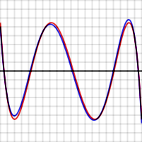
Error between optimal polynomial and log(x) (red), and Chebyshev approximation and log(x) (blue) over the interval [2, 4]. Vertical divisions are 10⁻⁵. Maximum error for the optimal polynomial is 6.07 x 10⁻⁵.

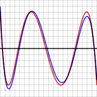
Error between optimal polynomial and exp(x) (red), and Chebyshev approximation and exp(x) (blue) over the interval [−1, 1]. Vertical divisions are 10⁻⁴. Maximum error for the optimal polynomial is 5.47 x 10⁻⁴.

Optimal polynomials

Once the domain (typically an interval) and degree of the polynomial are chosen, the polynomial itself is chosen in such a way as to minimize the worst-case error. That is, the goal is to minimize the maximum value of \( \mid P(x)-f(x)\mid \) , where P(x) is the approximating polynomial, f(x) is the actual function, and x varies over the chosen interval. For well-behaved functions, there exists an Nth-degree polynomial that will lead to an error curve that oscillates back and forth between \( +\varepsilon \) and \( -\varepsilon \) a total of N+2 times, giving a worst-case error of \varepsilon. It is seen that an Nth-degree polynomial can interpolate N+1 points in a curve. Such a polynomial is always optimal. It is possible to make contrived functions f(x) for which no such polynomial exists, but these occur rarely in practice.

For example the graphs shown to the right show the error in approximating log(x) and exp(x) for N = 4. The red curves, for the optimal polynomial, are level, that is, they oscillate between \( +\varepsilon \) and - \( \varepsilon \) exactly. Note that, in each case, the number of extrema is N+2, that is, 6. Two of the extrema are at the end points of the interval, at the left and right edges of the graphs.

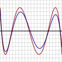
Error P(x) − f(x) for level polynomial (red), and for purported better polynomial (blue)

To prove this is true in general, suppose P is a polynomial of degree N having the property described, that is, it gives rise to an error function that has N + 2 extrema, of alternating signs and equal magnitudes. The red graph to the right shows what this error function might look like for N = 4. Suppose Q(x) (whose error function is shown in blue to the right) is another N-degree polynomial that is a better approximation to f than P. In particular, Q is closer to f than P for each value xi where an extreme of P−f occurs, so

\( |Q(x_i)-f(x_i)|<|P(x_i)-f(x_i)|. \)

When a maximum of P−f occurs at xi, then

\( Q(x_i)-f(x_i)\le|Q(x_i)-f(x_i)|<|P(x_i)-f(x_i)|=P(x_i)-f(x_i), \)

And when a minimum of P−f occurs at xi, then

\( f(x_i)-Q(x_i)\le|Q(x_i)-f(x_i)|<|P(x_i)-f(x_i)|=f(x_i)-P(x_i). \)

So, as can be seen in the graph, [P(x) − f(x)] − [Q(x) − f(x)] must alternate in sign for the N + 2 values of xi. But [P(x) − f(x)] − [Q(x) − f(x)] reduces to P(x) − Q(x) which is a polynomial of degree N. This function changes sign at least N+1 times so, by the Intermediate value theorem, it has N+1 zeroes, which is impossible for a polynomial of degree N.

Chebyshev approximation

One can obtain polynomials very close to the optimal one by expanding the given function in terms of Chebyshev polynomials and then cutting off the expansion at the desired degree. This is similar to the Fourier analysis of the function, using the Chebyshev polynomials instead of the usual trigonometric functions.

If one calculates the coefficients in the Chebyshev expansion for a function:

\( f(x) \sim \sum_{i=0}^\infty c_i T_i(x) \)

and then cuts off the series after the \( T_N \) term, one gets an Nth-degree polynomial approximating f(x).

The reason this polynomial is nearly optimal is that, for functions with rapidly converging power series, if the series is cut off after some term, the total error arising from the cutoff is close to the first term after the cutoff. That is, the first term after the cutoff dominates all later terms. The same is true if the expansion is in terms of Chebyshev polynomials. If a Chebyshev expansion is cut off after \(T_N \) , the error will take a form close to a multiple of \( T_{N+1} \) . The Chebyshev polynomials have the property that they are level – they oscillate between +1 and −1 in the interval [−1, 1]. T_{N+1} has N+2 level extrema. This means that the error between f(x) and its Chebyshev expansion out to T_N is close to a level function with N+2 extrema, so it is close to the optimal Nth-degree polynomial.

In the graphs above, note that the blue error function is sometimes better than (inside of) the red function, but sometimes worse, meaning that it is not quite the optimal polynomial. Note also that the discrepancy is less serious for the exp function, which has an extremely rapidly converging power series, than for the log function.

Chebyshev approximation is the basis for Clenshaw–Curtis quadrature, a numerical integration technique.
Remez' algorithm

The Remez algorithm (sometimes spelled Remes) is used to produce an optimal polynomial P(x) approximating a given function f(x) over a given interval. It is an iterative algorithm that converges to a polynomial that has an error function with N+2 level extrema. By the theorem above, that polynomial is optimal.

Remez' algorithm uses the fact that one can construct an Nth-degree polynomial that leads to level and alternating error values, given N+2 test points.

Given N+2 test points \( x_1, x_2, ... x_{N+2} \) (where \( x_1 \) and \( x_{N+2} \) are presumably the end points of the interval of approximation), these equations need to be solved:

\( P(x_1) - f(x_1) = + \varepsilon\, \)
\( P(x_2) - f(x_2) = - \varepsilon\, \)
\( P(x_3) - f(x_3) = + \varepsilon\, \)
\( \vdots \)
\( P(x_{N+2}) - f(x_{N+2}) = \pm \varepsilon.\, \)

The right-hand sides alternate in sign.

That is,

\( P_0 + P_1 x_1 + P_2 x_1^2 + P_3 x_1^3 + \dots + P_N x_1^N - f(x_1) = + \varepsilon\, \)
\( \( P_0 + P_1 x_2 + P_2 x_2^2 + P_3 x_2^3 + \dots + P_N x_2^N - f(x_2) = - \varepsilon\, \)
\vdots \)

Since \( x_1, ..., x_{N+2} \) were given, all of their powers are known, and \(f(x_1), ..., f(x_{N+2}) \) are also known. That means that the above equations are just N+2 linear equations in the N+2 variables \(P_0, P_1, ..., P_N \) , and \varepsilon. Given the test points \(x_1, ..., x_{N+2} \) , one can solve this system to get the polynomial P and the number \( \varepsilon. \)

The graph below shows an example of this, producing a fourth-degree polynomial approximating \( e^x \) over [−1, 1]. The test points were set at −1, −0.7, −0.1, +0.4, +0.9, and 1. Those values are shown in green. The resultant value of \varepsilon is 4.43 x 10−4

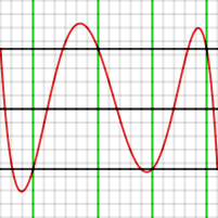
Error of the polynomial produced by the first step of Remez' algorithm, approximating e^x over the interval [−1, 1]. Vertical divisions are 10⁻⁴.

Note that the error graph does indeed take on the values \pm \varepsilon at the six test points, including the end points, but that those points are not extrema. If the four interior test points had been extrema (that is, the function P(x)f(x) had maxima or minima there), the polynomial would be optimal.

The second step of Remez' algorithm consists of moving the test points to the approximate locations where the error function had its actual local maxima or minima. For example, one can tell from looking at the graph that the point at −0.1 should have been at about −0.28. The way to do this in the algorithm is to use a single round of Newton's method. Since one knows the first and second derivatives of P(x)−f(x), one can calculate approximately how far a test point has to be moved so that the derivative will be zero.

Calculating the derivatives of a polynomial is straightforward. One must also be able to calculate the first and second derivatives of f(x). Remez' algorithm requires an ability to calculate \(f(x)\,, f'(x)\,, \) and f''(x)\, to extremely high precision. The entire algorithm must be carried out to higher precision than the desired precision of the result.

After moving the test points, the linear equation part is repeated, getting a new polynomial, and Newton's method is used again to move the test points again. This sequence is continued until the result converges to the desired accuracy. The algorithm converges very rapidly. Convergence is quadratic for well-behaved functions—if the test points are within \( 10^{-15} \) of the correct result, they will be approximately within \(10^{-30} \) of the correct result after the next round.

Remez' algorithm is typically started by choosing the extrema of the Chebyshev polynomial \(T_{N+1} \) as the initial points, since the final error function will be similar to that polynomial.

Main journals

Journal of Approximation Theory
Constructive Approximation
East Journal on Approximations

.

Approximation theory

References

N. I. Achiezer (Akhiezer), Theory of approximation, Translated by Charles J. Hyman Frederick Ungar Publishing Co., New York 1956 x+307 pp.
A. F. Timan, Theory of approximation of functions of a real variable, 1963 ISBN 0-486-67830-X
C. Hastings, Jr. Approximations for Digital Computers. Princeton University Press, 1955.
J. F. Hart, E. W. Cheney, C. L. Lawson, H. J. Maehly, C. K. Mesztenyi, J. R. Rice, H. C. Thacher Jr., C. Witzgall, Computer Approximations. Wiley, 1968, Lib. Cong. 67-23326.
L. Fox and I. B. Parker. "Chebyshev Polynomials in Numerical Analysis." Oxford University Press London, 1968.
Press, WH; Teukolsky, SA; Vetterling, WT; Flannery, BP (2007), "Section 5.8. Chebyshev Approximation", Numerical Recipes: The Art of Scientific Computing (3rd ed.), New York: Cambridge University Press, ISBN 978-0-521-88068-8
W. J. Cody Jr., W. Waite, Software Manual for the Elementary Functions. Prentice-Hall, 1980, ISBN 0-13-822064-6.
E. Remes [Remez], "Sur le calcul effectif des polynomes d'approximation de Tschebyscheff". 1934 C. R. Acad. Sci., Paris, 199, 337-340.
K.-G. Steffens, "The History of Approximation Theory: From Euler to Bernstein," Birkhauser, Boston 2006 ISBN 0-8176-4353-2.
T. Erdélyi, "Extensions of the Bloch-Pólya theorem on the number of distinct real zeros of polynomials", Journal de théorie des nombres de Bordeaux 20 (2008), 281–287.
T. Erdélyi, "The Remez inequality for linear combinations of shifted Gaussians", Math. Proc. Cambridge Phil. Soc. 146 (2009), 523–530.
L. N. Trefethen, "Approximation theory and approximation practice", SIAM 2013. [1]
External links
History of Approximation Theory (HAT)
Surveys in Approximation Theory (SAT)
Undergraduate Texts in Mathematics
Graduate Studies in Mathematics
Retrieved from "http://en.wikipedia.org/"
All text is available under the terms of the GNU Free Documentation License