.

The mathematics of pendulums are in general quite complicated. Simplifying assumptions can be made, which in the case of a simple pendulum allows the equations of motion to be solved analytically for small-angle oscillations.

Simple gravity pendulum

A simple pendulum is an idealization of a real pendulum using the following assumptions:

The rod or cord on which the bob swings is massless, inextensible and always remains taut;
Motion occurs only in two dimensions, i.e. the bob does not trace an ellipse but an arc.
The motion does not lose energy to friction or air resistance.

The differential equation which represents the motion of a simple pendulum is

\( {d^2\theta\over dt^2}+{g\over \ell} \sin\theta=0 \quad\quad\quad\quad\quad(1) \)

where g is acceleration due to gravity, \ell is the length of the pendulum, and θ is the angular displacement.
"Force" derivation of (1)
"Energy" derivation of (1)
Small-angle approximation

The differential equation given above is not easily solved. However adding a restriction to the size of the oscillation's amplitude gives a form whose solution can be easily obtained. If it is assumed that the angle is much less than 1 radian, or

\( \theta \ll 1\,, \)

then substituting for sin θ into (1) using the small-angle approximation,

\( \sin\theta\approx\theta\,,\)

yields the equation for a harmonic oscillator

\( {d^2\theta\over dt^2}+{g\over \ell}\theta=0.\)

The error due to the approximation is proportional to θ 3 (from the Maclaurin series for sin θ).

Given the initial conditions θ(0) = θ0 and dθ/dt(0) = 0 , the solution becomes,

\( \theta(t) = \theta_0\cos\left(\sqrt{g\over \ell\,}\,t\right) \quad\quad\quad\quad \theta_0 \ll 1.\)

The motion is simple harmonic motion where θ0 is the semi-amplitude of the oscillation (that is, the maximum angle between the rod of the pendulum and the vertical). The period of the motion, the time for a complete oscillation (outward and return) is

\( T_0 = 2\pi\sqrt{\frac{\ell}{g}} \quad\quad\quad\quad\quad \theta_0 \ll 1 \)

which is known as Christiaan Huygens's law for the period. Note that under the small-angle approximation, the period is independent of the amplitude θ0; this is the property of isochronism that Galileo discovered.
Rule of thumb for pendulum length

\( T_0 = 2\pi\sqrt{\frac{\ell}{g}} \) can be expressed as \( \ell = {\frac{g}{\pi^2}}\times{\frac{T_0^2}{4}}. \)

If SI units are used (i.e. measure in metres and seconds), and assuming the measurement is taking place on the Earth's surface, then \( \scriptstyle g\approx9.81 m/s^2 \), and \( \scriptstyle g/\pi^2\approx{1}\) (the exact figure is 0.994 to 3 decimal places).

Therefore a relatively reasonable approximation for the length and period are,

\( \ell\approx{\frac{T_0^2}{4}},
T_0 \approx 2 \sqrt{\ell} \)

Arbitrary-amplitude period

For amplitudes beyond the small angle approximation, one can compute the exact period by first inverting the equation for the angular velocity obtained from the energy method,
Figure 3. Deviation of the period from small-angle approximation.
Figure 4. Relative errors using the power series.

\( {dt\over d\theta} = \sqrt{\ell\over 2g}{1\over\sqrt{\cos\theta-\cos\theta_0}} \)

and then integrating over one complete cycle,

\( T = t(\theta_0\rightarrow0\rightarrow-\theta_0\rightarrow0\rightarrow\theta_0), \)

or twice the half-cycle

\( T = 2 t\left(\theta_0\rightarrow0\rightarrow-\theta_0\right), \)

or 4 times the quarter-cycle

\( T = 4 t\left(\theta_0\rightarrow0\right), \)

which leads to

\( T = 4\sqrt{\ell\over 2g}\int^{\theta_0}_0 {1\over\sqrt{\cos\theta-\cos\theta_0}}\,d\theta. \)

This integral can be re-written in the elliptic function of the first kind (also see Jacobi's elliptic functions), which gives little advantage since that form is also insoluble in terms of elementary functions,

\( T = 4\sqrt{\ell\over g}F\left(\csc{\theta_0\over2},{\theta_0\over 2}\right)\csc {\theta_0\over 2} \)

or more concisely, using the \( \theta\ \) , to \( u\, \) substitution, \( \sin{u} = \frac{\sin{\theta\over 2}}{\sin{\theta_0\over 2}} \)

\( T = 4\sqrt{\ell\over g}F\left(\sin{\theta_0\over 2}, {\pi \over 2} \right) \)

where \( F(k,\varphi) \) is Legendre's elliptic function of the first kind defined as

\( F(k,\varphi) = \int^\varphi_0 {1\over\sqrt{1-k^2\sin^2{u}}}\,du\,. \)

When \( \phi = \pi/2 , F(k,\varphi) \) is referred to as the complete elliptic function (or integral) of the first kind.

Figure 3 shows the deviation of T from T0, the period obtained from small-angle approximation.

Value for the complete elliptic function can be computed using the rapidly convergent, highly accurate arithmetic-geometric mean method (see elliptic integrals), or alternatively computed using the following series:

\( \begin{alignat}{2} T & = 2\pi \sqrt{\ell\over g} \left( 1+ \left( \frac{1}{2} \right)^2 \sin^2\left(\frac{\theta_0}{2}\right) + \left( \frac{1 \cdot 3}{2 \cdot 4} \right)^2 \sin^4\left(\frac{\theta_0}{2}\right) + \left( \frac {1 \cdot 3 \cdot 5}{2 \cdot 4 \cdot 6} \right)^2 \sin^6\left(\frac{\theta_0}{2}\right) + \cdots \right) \\ & = 2\pi \sqrt{\ell\over g} \cdot \sum_{n=0}^\infty \left[ \left ( \frac{(2 n)!}{( 2^n \cdot n! )^2} \right )^2 \cdot \sin^{2 n}\left(\frac{\theta_0}{2}\right) \right]. \end{alignat} \)

Figure 4 shows the relative errors using the power series. T0 is the linear approximation, and T2 to T10 include respectively the terms up to the 2nd to the 10th powers.

For a swing of exactly 180° the bob is balanced over its pivot point and so T = ∞.
Figure 5. Potential energy and phase portrait of a simple pendulum. Note that the x-axis, being angle, wraps onto itself after every 2π radians.

For example, the period of a pendulum of length 1 m on Earth (g = 9.80665 m/s2) at initial angle 10 degrees is \( 4\sqrt{1\ \mathrm{m}\over g}F\left({\sin {10^\circ\over 2}},{\pi\over2}\right) \approx 2.0102\ \mathrm{s} \) , where the linear approximation gives \( 2\pi \sqrt{1\ \mathrm{m}\over g} \approx 2.0064\ \mathrm{s}. \)
The difference (less than 0.2%) is much less than that caused by the variation of g with geographical location.

By using the following Maclaurin series:

\( F \left(x, {\pi \over 2} \right)={\pi \over 2} \left( 1 + \frac{1}{4}x^2 + \frac{9}{64}x^4 + \frac{25}{256}x^6 + \frac{1225}{16384}x^8 + \cdots\right) \)

\( \sin \left({\theta_0 \over 2}\right)=\left(\frac{1}{2}\theta_0 - \frac{1}{48}\theta_0^3 + \frac{1}{3840}\theta_0^5 - \frac{1}{645120}\theta_0^7 + \cdots\right) \)

The equivalent power series is:[1]

\( \begin{alignat}{2} T & = 2\pi \sqrt{\ell\over g} \left( 1+ \frac{1}{16}\theta_0^2 + \frac{11}{3072}\theta_0^4 + \frac{173}{737280}\theta_0^6 + \frac{22931}{1321205760}\theta_0^8 + \frac{1319183}{951268147200}\theta_0^{10} + \frac{233526463}{2009078326886400}\theta_0^{12} + . . . \right) \end{alignat} \)

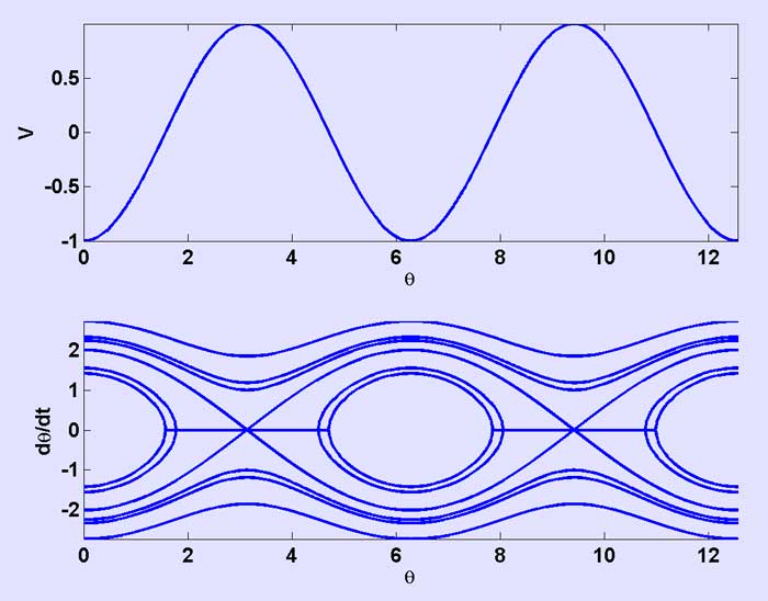
Figure 5. Potential energy and phase portrait of a simple pendulum. Note that the x-axis, being angle, wraps onto itself after every 2π radians.

Examples

Compound pendulum

A compound pendulum (or physical pendulum) is one where the rod is not massless, and may have extended size; that is, an arbitrarily shaped rigid body swinging by a pivot. In this case the pendulum's period depends on its moment of inertia I around the pivot point.

The equation of torque gives:

\( \tau = I \alpha\, \)

where:

\( \alpha \) is the angular acceleration.
\( \tau \) is the torque

The torque is generated by gravity so:

\( \tau = - m g L \sin\theta\, \)

where:

L is the distance from the pivot to the center of mass of the pendulum
θ is the angle from the vertical

Hence, under the small-angle approximation \( \scriptstyle \sin \theta \approx \theta\,, \)

\( \alpha \approx \frac{mgL \theta} {I} \)

This is of the same form as the conventional simple pendulum and this gives a period of:

\( T = 2 \pi \sqrt{\frac{I} {mgL}} \) [2]

And a frequency of:

\( f = \frac{1}{T} = \frac{1}{2\pi} \sqrt{\frac{mgL}{I}} \)

Physical interpretation of the imaginary period

The Jacobian elliptic function that expresses the position of a pendulum as a function of time is a doubly periodic function with a real period and an imaginary period. The real period is of course the time it takes the pendulum to go through one full cycle. Paul Appell pointed out a physical interpretation of the imaginary period:[3] if θ0 is the maximum angle of one pendulum and 180° − θ0 is the maximum angle of another, then the real period of each is the magnitude of the imaginary period of the other.
See also

Blackburn pendulum
Conical pendulum
Double pendulum
Inverted pendulum
Spring pendulum
Mathieu function
Pendulum equations (software)

References

^ Nelson, Robert; M. G. Olsson (February 1986). "The pendulum — Rich physics from a simple system". American Journal of Physics 54 (2): pp. 112–121. doi:10.1119/1.14703. Retrieved 2012-4-30.
^ Physical Pendulum
^ Paul Appell, "Sur une interprétation des valeurs imaginaires du temps en Mécanique", Comptes Rendus Hebdomadaires des Scéances de l'Académie des Sciences, volume 87, number 1, July, 1878