|
|
EQUATION (from Lat. aequatio, aequare, to equalize), an expression or statement of the equality of two quantities. Mathematical equivalence is denoted by the sign =, a symbol invented by Robert Recorde (1510-1558), who considered that nothing could be more equal than two equal and parallel straight lines. An equation states an equality existing between two classes of quantities, distinguished as known and unknown; these correspond to the data of a problem and the thing sought. It is the purpose of the mathematician to state the unknowns separately in terms of the knowns; this is called solving the equation, and the values of the unknowns so obtained are called the roots or solutions. The unknowns are usually denoted by the terminal letters, ... x, y, z, of the alphabet, and the knowns are either actual numbers or are represented by the literals a, b, c, &c..., i.e. the introductory letters of the alphabet. Any number or literal which expresses what multiple of term occurs in an equation is called the coefficient of that term; and the term which does not contain an unknown is called the absolute term. The degree of an equation is equal to the greatest index of an unknown in the equation, or to the greatest sum of the indices of products of unknowns. If each term has the sum of its indices the same, the equation is said to be homogeneous. These definitions are exemplified in the equations:—
In (1) the unknown is x, and the knowns a, b, c; the coefficients of x² and x are a and 2b; the absolute term is c, and the degree is 2. In (2) the unknowns are x and y, and the known a; the degree is 3, i.e. the sum of the indices in the term xy². (3) is a homogeneous equation of the second degree in x and y. Equations of the first degree are called simple or linear; of the second, quadratic; of the third, cubic; of the fourth, biquadratic; of the fifth, quintic, and so on. Of equations containing only one unknown the number of roots equals the degree of the equation; thus a simple equation has one root, a quadratic two, a cubic three, and so on. If one equation be given containing two unknowns, as for example ax + by = c or ax² + by² = c, it is seen that there are an infinite number of roots, for we can give x, say, any value and then determine the corresponding value of y; such an equation is called indeterminate; of the examples chosen the first is a linear and the second a quadratic indeterminate equation. In general, an indeterminate equation results when the number of unknowns exceeds by unity the number of equations. If, on the other hand, we have two equations connecting two unknowns, it is possible to solve the equations separately for one unknown, and then if we equate these values we obtain an equation in one unknown, which is soluble if its degree does not exceed the fourth. By substituting these values the corresponding values of the other unknown are determined. Such equations are called simultaneous; and a simultaneous system is a series of equations equal in number to the number of unknowns. Such a system is not always soluble, for it may happen that one equation is implied by the others; when this occurs the system is called porismatic or poristic. An identity differs from an equation inasmuch as it cannot be solved, the terms mutually cancelling; for example, the expression x² − a² = (x − a)(x + a) is an identity, for on reduction it gives 0 = 0. It is usual to employ the sign ≡ to express this relation. An equation admits of description in two ways:—(1) It may be regarded purely as an algebraic expression, or (2) as a geometrical locus. In the first case there is obviously no limit to the number of unknowns and to the degree of the equation; and, consequently, this aspect is the most general. In the second case the number of unknowns is limited to three, corresponding to the three dimensions of space; the degree is unlimited as before. It must be noticed, however, that by the introduction of appropriate hyperspaces, i.e. of degree equal to the number of unknowns, any equation theoretically admits of geometrical visualization, in other words, every equation may be represented by a geometrical figure and every geometrical figure by an equation. Corresponding to these two aspects, there are two typical methods by which equations can be solved, viz. the algebraic and geometric. The former leads to exact results, or, by methods of approximation, to results correct to any required degree of accuracy. The latter can only yield approximate values: when theoretically exact constructions are available there is a source of error in the draughtsmanship, and when the constructions are only approximate, the accuracy of the results is more problematical. The geometric aspect, however, is of considerable value in discussing the theory of equations. History.—There is little doubt that the earliest solutions of equations are given, in the Rhind papyrus, a hieratic document written some 2000 years before our era. The problems solved were of an arithmetical nature, assuming such forms as “a mass and its 1⁄7th makes 19.” Calling the unknown mass x, we have given x + 1⁄7 x = 19, which is a simple equation. Arithmetical problems also gave origin to equations involving two unknowns; the early Greeks were familiar with and solved simultaneous linear equations, but indeterminate equations, such, for instance, as the system given in the “cattle problem” of Archimedes, were not seriously studied until Diophantus solved many particular problems. Quadratic equations arose in the Greek investigations in the doctrine of proportion, and 710 although they were presented and solved in a geometrical form, the methods employed have no relation to the generalized conception of algebraic geometry which represents a curve by an equation and vice versa. The simplest quadratic arose in the construction of a mean proportional (x) between two lines (a, b), or in the construction of a square equal to a given rectangle; for we have the proportion a:x = x:b; i.e. x² = ab. A more general equation, viz. x² − ax + a² = 0, is the algebraic equivalent of the problem to divide a line in medial section; this is solved in Euclid, ii. 11. It is possible that Diophantus was in possession of an algebraic solution of quadratics; he recognized, however, only one root, the interpretation of both being first effected by the Hindu Bhaskara. A simple cubic equation was presented in the problem of finding two mean proportionals, x, y, between two lines, one double the other. We have a:x = x:y = y:2a, which gives x² = ay and xy = 2a²; eliminating y we obtain x³ = 2a³, a simple cubic. The Greeks could not solve this equation, which also arose in the problems of duplicating a cube and trisecting an angle, by the ruler and compasses, but only by mechanical curves such as the cissoid, conchoid and quadratrix. Such solutions were much improved by the Arabs, who also solved both cubics and biquadratics by means of intersecting conics; at the same time, they developed methods, originated by Diophantus and improved by the Hindus, for finding approximate roots of numerical equations by algebraic processes. The algebraic solution of the general cubic and biquadratic was effected in the 16th century by S. Ferro, N. Tartaglia, H. Cardan and L. Ferrari (see Algebra: History). Many fruitless attempts were made to solve algebraically the quintic equation until P. Ruffini and N.H. Abel proved the problem to be impossible; a solution involving elliptic functions has been given by C. Hermite and L. Kronecker, while F. Klein has given another solution. In the geometric treatment of equations the Greeks and Arabs based their constructions upon certain empirically deduced properties of the curves and figures employed. Knowing various metrical relations, generally expressed as proportions, it was found possible to solve particular equations, but a general method was wanting. This lacuna was not filled until the 17th century, when Descartes discovered the general theory which explained the nature of such solutions, in particular those wherein conics were employed, and, in addition, established the most important facts that every equation represents a geometrical locus, and conversely. To represent equations containing two unknowns, x, y, he chose two axes of reference mutually perpendicular, and measured x along the horizontal axis and y along the vertical. Then by the methods described in the article Geometry: Analytical, he showed that—(1) a linear equation represents a straight line, and (2) a quadratic represents a conic. If the equation be homogeneous or break up into factors, it represents a number of straight lines in the first case, and the loci corresponding to the factors in the second. The solution of simultaneous equations is easily seen to be the values of x, y corresponding to the intersections of the loci. It follows that there is only one value of x, y which satisfies two linear equations, since two lines intersect in one point only; two values which satisfy a linear and quadratic, since a line intersects a conic in two points; and four values which satisfy two quadratics, since two conics intersect in four points. It may happen that the curves do not actually intersect in the theoretical maximum number of points; the principle of continuity (see Geometrical Continuity) shows us that in such cases some of the roots are imaginary. To represent equations involving three unknowns x, y, z, a third axis is introduced, the z-axis, perpendicular to the plane xy and passing through the intersection of the lines x, y. In this notation a linear equation represents a plane, and two linear simultaneous equations represent a line, i.e. the intersection of two planes; a quadratic equation represents a surface of the second degree. In order to graphically consider equations containing only one unknown, it is convenient to equate the terms to y; i.e. if the equation be ƒ(x) = 0, we take y = ƒ(x) and construct this curve on rectangular Cartesian co-ordinates by determining the values of y which correspond to chosen values of x, and describing a curve through the points so obtained. The intersections of the curve with the axis of x gives the real roots of the equation; imaginary roots are obviously not represented. In this article we shall treat of: (1) Simultaneous equations, (2) indeterminate equations, (3) cubic equations, (4) biquadratic equations, (5) theory of equations. Simple, linear simultaneous and quadratic equations are treated in the article Algebra; for differential equations see Differential Equations. I. Simultaneous Equations. Simultaneous equations which involve the second and higher powers of the unknown may be impossible of solution. No general rules can be given, and the solution of any particular problem will largely depend upon the student’s ingenuity. Here we shall only give a few typical examples. 1. Equations which may be reduced to linear equations.—Ex. To solve x(x − a) = yz, y (y − b) = zx, z (z − c) = xy. Multiply the equations by y, z and x respectively, and divide the sum by xyz; then
(1).
Multiply by z, x and y, and divide the sum by xyz; then
(2).
From (1) and (2) by cross multiplication we obtain
(3).
Substituting for x, y and z in x (x − a) = yz we obtain
and therefore x, y and z are known from (3). The same artifice solves the equations x² − yz = a, y² − xz = b, z² − xy = c. 2. Equations which are homogeneous and of the same degree.—These equations can be solved by substituting y = mx. We proceed to explain the method by an example. Ex. To solve 3x² + xy + y² = 15, 31xy − 3x² − 5y² = 45. Substituting y = mx in both these equations, and then dividing, we obtain 31m − 3 − 5m² = 3 (3 + m + m²) or 8m² − 28m + 12 = 0. The roots of this quadratic are m = ½ or 3, and therefore 2y = x, or y = 3x. Taking 2y = x and substituting in 3x² + xy + y² = 0, we obtain y² (12 + 2 + 1) = 15; ∴ y² = 1, which gives y = ±1, x = ±2. Taking the second value, y = 3x, and substituting for y, we obtain x² (3 + 3 + 9) = 15; ∴ x² = 1, which gives x = ±1, y = ±3. Therefore the solutions are x = ±2, y = ±1 and x = ±1, y = ±3. Other artifices have to be adopted to solve other forms of simultaneous equations, for which the reader is referred to J.J. Milne, Companion to Weekly Problem Papers. II. Indeterminate Equations. 1. When the number of unknown quantities exceeds the number of equations, the equations will admit of innumerable solutions, and are therefore said to be indeterminate. Thus if it be required to find two numbers such that their sum be 10, we have two unknown quantities x and y, and only one equation, viz. x + y = 10, which may evidently be satisfied by innumerable different values of x and y, if fractional solutions be admitted. It is, however, usual, in such questions as this, to restrict values of the numbers sought to positive integers, and therefore, in this case, we can have only these nine solutions,
which indeed may be reduced to five; for the first four become the same as the last four, by simply changing x into y, and the contrary. This branch of analysis was extensively studied by Diophantus, and is sometimes termed the Diophantine Analysis. 2. Indeterminate problems are of different orders, according to the dimensions of the equation which is obtained after all the unknown quantities but two have been eliminated by means of the given equations. Those of the first order lead always to equations of the form ax ± by = ±c, where a, b, c denote given whole numbers, and x, y two numbers to be found, so that both may be integers. That this condition may be fulfilled, it is necessary that the coefficients a, b have no common divisor which is not also a divisor of c; for if a = md and b = me, then ax + by = mdx + mey = c, and dx + ey = c/m; but d, e, x, y are supposed to be whole numbers, therefore c/m is a whole number; hence m must be a divisor of c. Of the four forms expressed by the equation ax ± by = ±c, it is obvious that ax + by = −c can have no positive integral solutions. Also ax − by = −c is equivalent to by − ax = c, and so we have only to consider the forms ax ± by = c. Before proceeding to the general solution of these equations we will give a numerical example. To solve 2x + 3y = 25 in positive integers. From the given equation 711 we have x = (25 − 3y) / 2 = 12 − y − (y − 1) / 2. Now, since x must be a whole number, it follows that (y − 1)/2 must be a whole number. Let us assume (y − 1) / 2 = z, then y = 1 + 2z; and x = 11 − 3z, where z might be any whole number whatever, if there were no limitation as to the signs of x and y. But since these quantities are required to be positive, it is evident, from the value of y, that z must be either 0 or positive, and from the value of x, that it must be less than 4; hence z may have these four values, 0, 1, 2, 3.
3. We shall now give the solution of the equation ax − by = c in positive integers. Convert a/b into a continued fraction, and let p/q be the convergent immediately preceding a/b, then aq − bp = ±1 (see Continued Fraction). (α) If aq − bp = 1, the given equation may be written ax − by = c (aq − bp); Since a and b are prime to one another, then x − cq must be divisible by b and y − cp by a; hence (x − cq) / b = (y − cq) / a = t. That is, x = bt + cq and y = at + cp. Positive integral solutions, unlimited in number, are obtained by giving t any positive integral value, and any negative integral value, so long as it is numerically less than the smaller of the quantities cq/b, cp/a; t may also be zero. (β) If aq − bp = −1, we obtain x = bt − cq, y = at − cp, from which positive integral solutions, again unlimited in number, are obtained by giving t any positive integral value which exceeds the greater of the two quantities cq/b, cp/a. If a or b is unity, a/b cannot be converted into a continued fraction with unit numerators, and the above method fails. In this case the solutions can be derived directly, for if b is unity, the equation may be written y = ax − c, and solutions are obtained by giving x positive integral values greater than c/a. 4. To solve ax + by = c in positive integers. Converting a b into a continued fraction and proceeding as before, we obtain, in the case of aq − bp = 1, x = cq − bt, y = at − cp. Positive integral solutions are obtained by giving t positive integral values not less than cp/a and not greater than cq/b. In this case the number of solutions is limited. If aq − bp = −1 we obtain the general solution x = bt − cq, y = cp − at, which is of the same form as in the preceding case. For the determination of the number of solutions the reader is referred to H.S. Hall and S.R. Knight’s Higher Algebra, G. Chrystal’s Algebra, and other text-books. 5. If an equation were proposed involving three unknown quantities, as ax + by + cz = d, by transposition we have ax + by = d − cz, and, putting d − cz = c′, ax + by = c′. From this last equation we may find values of x and y of this form, x = mr + nc′, y = mr + n′c′, where z and r may be taken at pleasure, except in so far as the values of x, y, z may be required to be all positive; for from such restriction the values of z and r may be confined within certain limits to be determined from the given equation. For more advanced treatment of linear indeterminate equations see Combinatorial Analysis. 6. We proceed to indeterminate problems of the second degree: limiting ourselves to the consideration of the formula y² = a + bx + cx², where x is to be found, so that y may be a rational quantity. The possibility of rendering the proposed formula a square depends altogether upon the coefficients a, b, c; and there are four cases of the problem, the solution of each of which is connected with some peculiarity in its nature. Case 1. Let a be a square number; then, putting g² for a, we have y² = g² + bx + cx². Suppose √(g² + bx + cx²) = g + mx; then g² + bx + cx² = g² + 2gmx + m²x², or bx + cx² = 2gmx + m²x², that is, b + cx = 2gm + m²x; hence
Case 2. Let c be a square number = g²; then, putting √(a + bx + g²x²) = m + gx, we find a + bx + g²x² = m² + 2mgx + g²x², or a + bx = m² + 2mgx; hence we find
Case 3. When neither a nor c is a square number, yet if the expression a + bx + cx² can be resolved into two simple factors, as f + gx and h + kx, the irrationality may be taken away as follows:— Assume √(a + bx + cx²) = √{ (f + gx) (h + kx) } = m (f + gx), then (f + gx) (h + kx) = m² (f + gx)², or h + kx = m² (f + gx); hence we find
and in all these formulae m may be taken at pleasure. Case 4. The expression a + bx + cx² may be transformed into a square as often as it can be resolved into two parts, one of which is a complete square, and the other a product of two simple factors; for then it has this form, p² + qr, where p, q and r are quantities which contain no power of x higher than the first. Let us assume √(p² + qr) = p + mq; thus we have p² + qr = p² + 2mpq + m²q² and r = 2mp + m²q, and as this equation involves only the first power of x, we may by proper reduction obtain from it rational values of x and y, as in the three foregoing cases. The application of the preceding general methods of resolution to any particular case is very easy; we shall therefore conclude with a single example. Ex. It is required to find two square numbers whose sum is a given square number. Let a² be the given square number, and x², y² the numbers required; then, by the question, x² + y² = a², and y = √(a² − x²). This equation is evidently of such a form as to be resolvable by the method employed in case 1. Accordingly, by comparing √(a² − x²) with the general expression √(g² + bx + cx²), we have g = a, b = 0, c = −1, and substituting these values in the formulae, and also −n for +m, we find
If a = n² + 1, there results x = 2n, y = n² − 1, a = n² + 1. Hence if r be an even number, the three sides of a rational right-angled triangle are r, (½ r)² − 1, (½ r)² + 1. If r be an odd number, they become (dividing by 2) r, ½ (r² − 1), ½ (r² + 1). For example, if r = 4, 4, 4 − 1, 4 + 1, or 4, 3, 5, are the sides of a right-angled triangle; if r = 7, 7, 24, 25 are the sides of a right-angled triangle. III. Cubic Equations. 1. Cubic equations, like all equations above the first degree, are divided into two classes: they are said to be pure when they contain only one power of the unknown quantity; and adfected when they contain two or more powers of that quantity. Pure cubic equations are therefore of the form x³ = r; and hence it appears that a value of the simple power of the unknown quantity may always be found without difficulty, by extracting the cube root of each side of the equation. Let us consider the equation x³ − c³ = 0 more fully. This is decomposable into the factors x − c = 0 and x² + cx + c² = 0. The roots of this quadratic equation are ½ (−1 ± √−3) c, and we see that the equation x³ = c³ has three roots, namely, one real root c, and two imaginary roots ½ (−1 ± √−3) c. By making c equal to unity, we observe that ½ (−1 ± √−3) are the imaginary cube roots of unity, which are generally denoted by ω and ω², for it is easy to show that (½ (−1 − √−3))² = ½ (−1 + √−3). 2. Let us now consider such cubic equations as have all their terms, and which are therefore of this form, x³ + Ax² + Bx + C = 0, where A, B and C denote known quantities, either positive or negative. This equation may be transformed into another in which the second term is wanting by the substitution x = y − A/3. This transformation is a particular case of a general theorem. Let xn + Axn−1 + Bxn−2 ... = 0. Substitute x = y + h; then (y + h)n + A (y + h)n−1 ... = 0. Expand each term by the binomial theorem, and let us fix our attention on the coefficient of yn−1. By this process we obtain 0 = yn + yn−1(A + nh) + terms involving lower powers of y. Now h can have any value, and if we choose it so that A + nh = 0, then the second term of our derived equation vanishes. Resuming, therefore, the equation y³ + qy + r = 0, let us suppose y = v + z; we then have y³ = v³ + z³ + 3vz (v + z) = v³ + z³ + 3vzy, and the original equation becomes v³ + z³ + (3vz + q) y + r = 0. Now v and z are any two quantities subject to the relation y = v + z, and if we suppose 3vz + q = 0, they are completely determined. This leads to v³ + z³ + r = 0 and 3vz + q = 0. Therefore v³ and z³ are the roots of the quadratic t² + rt − q²/27 = 0. Therefore
Thus we have obtained a value of the unknown quantity y, in terms of the known quantities q and r; therefore the equation is resolved. 3. But this is only one of three values which y may have. Let us, for the sake of brevity, put A = −½ r + √(1⁄27 q³ + ¼ r²), B = −½ r − √(1⁄27 q³ + ¼ r²),
Then, from what has been shown (§ 1), it is evident that v and z have each these three values, v = 3√A, v = α3√A, v = β3√A; To determine the corresponding values of v and z, we must consider that vz = −1⁄3 q = 3√(AB). Now if we observe that αβ = 1, it will immediately appear that v + z has these three values, v + z = 3√A + 3√B, which are therefore the three values of y. The first of these formulae is commonly known by the name of Cardan’s rule (see Algebra: History). The formulae given above for the roots of a cubic equation may be put under a different form, better adapted to the purposes of arithmetical calculation, as follows:—Because vz = −1⁄3 q, therefore z = −1⁄3q × 1/v = −1⁄3 q / 3√A; hence v + z = 3√A − 1⁄3 q / 3√A: thus it appears that the three values of y may also be expressed thus: y = 3√A − 1⁄3 q / 3√A See below, Theory of Equations, §§ 16 et seq. IV. Biquadratic Equations. 1. When a biquadratic equation contains all its terms, it has this form, x4 + Ax³ + Bx² + Cx + D = 0, where A, B, C, D denote known quantities. We shall first consider pure biquadratics, or such as contain only the first and last terms, and therefore are of this form, x4 = b4. In this case it is evident that x may be readily had by two extractions of the square root; by the first we find x² = b², and by the second x = b. This, however, is only one of the values which x may have; for since x4 = b4, therefore x4 − b4 = 0; but x4 − b4 may be resolved into two factors x² − b² and x² + b², each of which admits of a similar resolution; for x² − b² = (x − b)(x + b) and x² + b² = (x − b√−1)(x + b√−1). Hence it appears that the equation x4 − b4 = 0 may also be expressed thus, (x − b) (x + b) (x − b√−1) (x + b√−1) = 0; so that x may have these four values, +b, −b, +b√−1, −b√−1, two of which are real, and the others imaginary. 2. Next to pure biquadratic equations, in respect of easiness of resolution, are such as want the second and fourth terms, and therefore have this form, x4 + qx² + s = 0. These may be resolved in the manner of quadratic equations; for if we put y = x², we have y² + qy + s = 0, from which we find y = ½ {−q ± √(q² − 4s) }, and therefore x = ±√½ {−q ± √(q² − 4s) }. 3. When a biquadratic equation has all its terms, its resolution may be always reduced to that of a cubic equation. There are various methods by which such a reduction may be effected. The following was first given by Leonhard Euler in the Petersburg Commentaries, and afterwards explained more fully in his Elements of Algebra. We have already explained how an equation which is complete in its terms may be transformed into another of the same degree, but which wants the second term; therefore any biquadratic equation may be reduced to this form, y4 + py² + qy + r = 0, where the second term is wanting, and where p, q, r denote any known quantities whatever. That we may form an equation similar to the above, let us assume y = √a + √b + √c, and also suppose that the letters a, b, c denote the roots of the cubic equation z³ + Pz² + Qz − R = 0; then, from the theory of equations we have a + b + c = −P, ab + ac + bc = Q, abc = R. We square the assumed formula y = √a + √b + √c, and obtain y² = a + b + c + 2(√ab + √ac + √bc); or, substituting −P for a + b + c, and transposing, y² + P = 2(√ab + √ac + √bc). Let this equation be also squared, and we have y4 + 2Py² + P² = 4 (ab + ac + bc) + 8 (√a²bc + √ab²c + √abc²); and since ab + ac + bc = Q, and √a²bc + √ab²c + √abc² = √abc (√a + √b + √c) = √R·y, the same equation may be expressed thus: y4 + 2Py² + P² = 4Q + 8√R·y. Thus we have the biquadratic equation y4 + 2Py² − 8√R·y + P² − 4Q = 0, one of the roots of which is y = √a + √b + √c, while a, b, c are the roots of the cubic equation z³ + Pz² + Qz − R = 0. 4. In order to apply this resolution to the proposed equation y4 + py² + qy + r = 0, we must express the assumed coefficients P, Q, R by means of p, q, r, the coefficients of that equation. For this purpose let us compare the equations y4 + py² + qy + r = 0, and it immediately appears that 2P = p, −8√R = q, P² − 4Q = r; and from these equations we find P = ½ p, Q = 1⁄16 (p² − 4r), R = 1⁄64 q². Hence it follows that the roots of the proposed equation are generally expressed by the formula y = √a + √b + √c; where a, b, c denote the roots of this cubic equation,
But to find each particular root, we must consider, that as the square root of a number may be either positive or negative, so each of the quantities √a, √b, √c may have either the sign + or − prefixed to it; and hence our formula will give eight different expressions for the root. It is, however, to be observed, that as the product of the three quantities √a, √b, √c must be equal to √R or to −1⁄8 q; when q is positive, their product must be a negative quantity, and this can only be effected by making either one or three of them negative; again, when q is negative, their product must be a positive quantity; so that in this case they must either be all positive, or two of them must be negative. These considerations enable us to determine that four of the eight expressions for the root belong to the case in which q is positive, and the other four to that in which it is negative. 5. We shall now give the result of the preceding investigation in the form of a practical rule; and as the coefficients of the cubic equation which has been found involve fractions, we shall transform it into another, in which the coefficients are integers, by supposing z = ¼ v. Thus the equation
becomes, after reduction, v³ + 2pv² + (p² − 4r) v − q² = 0; it also follows, that if the roots of the latter equation are a, b, c, the roots of the former are ¼ a, ¼ b, ¼ c, so that our rule may now be expressed thus: Let y4 + py² + qy + r = 0 be any biquadratic equation wanting its second term. Form this cubic equation v³ + 2pv² + (p² − 4r) v − q² = 0, and find its roots, which let us denote by a, b, c. Then the roots of the proposed biquadratic equation are,
See also below, Theory of Equations, § 17 et seq.
(X.)
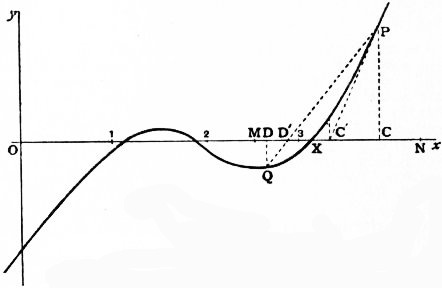
V. Theory of Equations. 1. In the subject “Theory of Equations” the term equation is used to denote an equation of the form xn − p1xn−1 ... ± pn = 0, where p1, p2 ... pn are regarded as known, and x as a quantity to be determined; for shortness the equation is written ƒ(x) = 0. The equation may be numerical; that is, the coefficients p1, p2n, ... pn are then numbers—understanding by number a quantity of the form α + βi (α and β having any positive or negative real values whatever, or say each of these is regarded as susceptible of continuous variation from an indefinitely large negative to an indefinitely large positive value), and i denoting √−1. Or the equation may be algebraical; that is, the coefficients are not then restricted to denote, or are not explicitly considered as denoting, numbers. 1. We consider first numerical equations. (Real theory, 2-6; Imaginary theory, 7-10.) Real Theory. 2. Postponing all consideration of imaginaries, we take in the first instance the coefficients to be real, and attend only to the real roots (if any); that is, p1, p2, ... pn are real positive or negative quantities, and a root a, if it exists, is a positive or negative quantity such that an − p1an−1 ... ± pn = 0, or say, ƒ(a) = 0. It is very useful to consider the curve y = ƒ(x),—or, what would come to the same, the curve Ay = ƒ(x),—but it is better to retain the first-mentioned form of equation, drawing, if need be, the ordinate y on a reduced scale. For instance, if the given equation be x³ − 6x² + 11x − 6.06 = 0,1 then the curve 713 y = x³ − 6x² + 11x − 6.06 is as shown in fig. 1, without any reduction of scale for the ordinate. It is clear that, in general, y is a continuous one-valued function of x, finite for every finite value of x, but becoming infinite when x is infinite; i.e., assuming throughout that the coefficient of xn is +1, then when x = ∞, y = +∞; but when x = −∞, then y = +∞ or −∞, according as n is even or odd; the curve cuts any line whatever, and in particular it cuts the axis (of x) in at most n points; and the value of x, at any point of intersection with the axis, is a root of the equation ƒ(x) = 0. If β, α are any two values of x (α > β, that is, α nearer +∞), then if ƒ(β), ƒ(α) have opposite signs, the curve cuts the axis an odd number of times, and therefore at least once, between the points x = β, x = α; but if ƒ(β), ƒ(α) have the same sign, then between these points the curve cuts the axis an even number of times, or it may be not at all. That is, ƒ(β), ƒ(α) having opposite signs, there are between the limits β, α an odd number of real roots, and therefore at least one real root; but ƒ(β), ƒ(α) having the same sign, there are between these limits an even number of real roots, or it may be there is no real root. In particular, by giving to β, α the values -∞, +∞ (or, what is the same thing, any two values sufficiently near to these values respectively) it appears that an equation of an odd order has always an odd number of real roots, and therefore at least one real root; but that an equation of an even order has an even number of real roots, or it may be no real root. If α be such that for x = or > a (that is, x nearer to +∞) ƒ(x) is always +, and β be such that for x = or < β (that is, x nearer to −∞) ƒ(x) is always −, then the real roots (if any) lie between these limits x = β, x = α; and it is easy to find by trial such two limits including between them all the real roots (if any). 3. Suppose that the positive value δ is an inferior limit to the difference between two real roots of the equation; or rather (since the foregoing expression would imply the existence of real roots) suppose that there are not two real roots such that their difference taken positively is = or < δ; then, γ being any value whatever, there is clearly at most one real root between the limits γ and γ + δ; and by what precedes there is such real root or there is not such real root, according as ƒ(γ), ƒ(γ + δ) have opposite signs or have the same sign. And by dividing in this manner the interval β to α into intervals each of which is = or < δ, we should not only ascertain the number of the real roots (if any), but we should also separate the real roots, that is, find for each of them limits γ, γ + δ between which there lies this one, and only this one, real root. In particular cases it is frequently possible to ascertain the number of the real roots, and to effect their separation by trial or otherwise, without much difficulty; but the foregoing was the general process as employed by Joseph Louis Lagrange even in the second edition (1808) of the Traité de la résolution des équations numériques;2 the determination of the limit δ had to be effected by means of the “equation of differences” or equation of the order ½ n(n − 1), the roots of which are the squares of the differences of the roots of the given equation, and the process is a cumbrous and unsatisfactory one. 4. The great step was effected by the theorem of J.C.F. Sturm (1835)—viz. here starting from the function ƒ(x), and its first derived function ƒ′(x), we have (by a process which is a slight modification of that for obtaining the greatest common measure of these two functions) to form a series of functions ƒ(x), ƒ′(x), ƒ2(x), ... ƒn(x) of the degrees n, n − 1, n − 2 ... 0 respectively,—the last term ƒn(x) being thus an absolute constant. These lead to the immediate determination of the number of real roots (if any) between any two given limits β, α; viz. supposing α > β (that is, α nearer to +∞), then substituting successively these two values in the series of functions, and attending only to the signs of the resulting values, the number of the changes of sign lost in passing from β to α is the required number of real roots between the two limits. In particular, taking β, α = −∞, +∞ respectively, the signs of the several functions depend merely on the signs of the terms which contain the highest powers of x, and are seen by inspection, and the theorem thus gives at once the whole number of real roots. And although theoretically, in order to complete by a finite number of operations the separation of the real roots, we still need to know the value of the before-mentioned limit δ; yet in any given case the separation may be effected by a limited number of repetitions of the process. The practical difficulty is when two or more roots are very near to each other. Suppose, for instance, that the theorem shows that there are two roots between 0 and 10; by giving to x the values 1, 2, 3, ... successively, it might appear that the two roots were between 5 and 6; then again that they were between 5.3 and 5.4, then between 5.34 and 5.35, and so on until we arrive at a separation; say it appears that between 5.346 and 5.347 there is one root, and between 5.348 and 5.349 the other root. But in the case in question δ would have a very small value, such as .002, and even supposing this value known, the direct application of the first-mentioned process would be still more laborious. 5. Supposing the separation once effected, the determination of the single real root which lies between the two given limits may be effected to any required degree of approximation either by the processes of W.G. Horner and Lagrange (which are in principle a carrying out of the method of Sturm’s theorem), or by the process of Sir Isaac Newton, as perfected by Joseph Fourier (which requires to be separately considered). First as to Horner and Lagrange. We know that between the limits β, α there lies one, and only one, real root of the equation; ƒ(β) and ƒ(α) have therefore opposite signs. Suppose any intermediate value is θ; in order to determine by Sturm’s theorem whether the root lies between β, θ, or between θ, α, it would be quite unnecessary to calculate the signs of ƒ(θ),ƒ′(θ), ƒ2(θ) ...; only the sign of ƒ(θ) is required; for, if this has the same sign as ƒ(β), then the root is between β, θ; if the same sign as ƒ(α), then the root is between θ, α. We want to make θ increase from the inferior limit β, at which ƒ(θ) has the sign of ƒ(β), so long as ƒ(θ) retains this sign, and then to a value for which it assumes the opposite sign; we have thus two nearer limits of the required root, and the process may be repeated indefinitely. Horner’s method (1819) gives the root as a decimal, figure by figure; thus if the equation be known to have one real root between 0 and 10, it is in effect shown say that 5 is too small (that is, the root is between 5 and 6); next that 5.4 is too small (that is, the root is between 5.4 and 5.5); and so on to any number of decimals. Each figure is obtained, not by the successive trial of all the figures which precede it, but (as in the ordinary process of the extraction of a square root, which is in fact Horner’s process applied to this particular case) it is given presumptively as the first figure of a quotient; such value may be too large, and then the next inferior integer must be tried instead of it, or it may require to be further diminished. And it is to be remarked that the process not only gives the approximate value α of the root, but (as in the extraction of a square root) it includes the calculation of the function ƒ(α), which should be, and approximately is, = 0. The arrangement of the calculations is very elegant, and forms an integral part of the actual method. It is to be observed that after a certain number of decimal places have been obtained, a good many more can be found by a mere division. It is in the progress tacitly assumed that the roots have been first separated. Lagrange’s method (1767) gives the root as a continued fraction a + 1/b + 1/c + ..., where a is a positive or negative integer (which may be = 0), but b, c, ... are positive integers. Suppose the roots have been separated; then (by trial if need be of consecutive integer values) the limits may be made to be consecutive integer numbers: say they are a, a + 1; the value of x is therefore = a + 1/y, where y is positive and greater than 1; from the given equation for x, writing therein x = a + 1/y, we form an equation of the same order for y, and this equation will have one, and only one, positive root greater than 1; hence finding for it the limits b, b + 1 (where b is = or > 1), we have y = b + 1/z, where z is positive and greater than 1; and so on—that is, we thus obtain the successive denominators b, c, d ... of the continued fraction. The method is theoretically very elegant, but the disadvantage is that it gives the result in the form of a continued fraction, which for the most part must ultimately be converted into a decimal. There is one advantage in the method, that a commensurable root (that is, a root equal to a rational fraction) is found accurately, since, when such root exists, the continued fraction terminates. 6. Newton’s method (1711), as perfected by Fourier(1831), may be 714 roughly stated as follows. If x = γ be an approximate value of any root, and γ + h the correct value, then ƒ(γ + h) = 0, that is,
and then, if h be so small that the terms after the second may be neglected, ƒ(γ) + hƒ′(γ) = 0, that is, h = {−ƒ(γ)/ƒ′(γ) }, or the new approximate value is x = γ − {ƒ(γ)/ƒ′(γ) }; and so on, as often as we please. It will be observed that so far nothing has been assumed as to the separation of the roots, or even as to the existence of a real root; γ has been taken as the approximate value of a root, but no precise meaning has been attached to this expression. The question arises, What are the conditions to be satisfied by γ in order that the process may by successive repetitions actually lead to a certain real root of the equation; or that, γ being an approximate value of a certain real root, the new value γ − {ƒ(γ)/ƒ′(γ) } may be a more approximate value.
Referring to fig. 1, it is easy to see that if OC represent the assumed value γ, then, drawing the ordinate CP to meet the curve in P, and the tangent PC′ to meet the axis in C′, we shall have OC′ as the new approximate value of the root. But observe that there is here a real root OX, and that the curve beyond X is convex to the axis; under these conditions the point C′ is nearer to X than was C; and, starting with C′ instead of C, and proceeding in like manner to draw a new ordinate and tangent, and so on as often as we please, we approximate continually, and that with great rapidity, to the true value OX. But if C had been taken on the other side of X, where the curve is concave to the axis, the new point C′ might or might not be nearer to X than was the point C; and in this case the method, if it succeeds at all, does so by accident only, i.e. it may happen that C′ or some subsequent point comes to be a point C, such that CO is a proper approximate value of the root, and then the subsequent approximations proceed in the same manner as if this value had been assumed in the first instance, all the preceding work being wasted. It thus appears that for the proper application of the method we require more than the mere separation of the roots. In order to be able to approximate to a certain root α, = OX, we require to know that, between OX and some value ON, the curve is always convex to the axis (analytically, between the two values, ƒ(x) and ƒ″(x) must have always the same sign). When this is so, the point C may be taken anywhere on the proper side of X, and within the portion XN of the axis; and the process is then the one already explained. The approximation is in general a very rapid one. If we know for the required root OX the two limits OM, ON such that from M to X the curve is always concave to the axis, while from X to N it is always convex to the axis,—then, taking D anywhere in the portion MX and (as before) C in the portion XN, drawing the ordinates DQ, CP, and joining the points P, Q by a line which meets the axis in D′, also constructing the point C′ by means of the tangent at P as before, we have for the required root the new limits OD′, OC′; and proceeding in like manner with the points D′, C′, and so on as often as we please, we obtain at each step two limits approximating more and more nearly to the required root OX. The process as to the point D′, translated into analysis, is the ordinate process of interpolation. Suppose OD = β, OC = α, we have approximately ƒ(β + h) = ƒ(β) + h{ƒ(α) − ƒ(β) } / (α − β), whence if the root is β + h then h = − (α − β)ƒ(β) / {ƒ(α) − ƒ(β) }. Returning for a moment to Horner’s method, it may be remarked that the correction h, to an approximate value α, is therein found as a quotient the same or such as the quotient ƒ(α) ÷ ƒ′(α) which presents itself in Newton’s method. The difference is that with Horner the integer part of this quotient is taken as the presumptive value of h, and the figure is verified at each step. With Newton the quotient itself, developed to the proper number of decimal places, is taken as the value of h; if too many decimals are taken, there would be a waste of work; but the error would correct itself at the next step. Of course the calculation should be conducted without any such waste of work. Imaginary Theory. 7. It will be recollected that the expression number and the correlative epithet numerical were at the outset used in a wide sense, as extending to imaginaries. This extension arises out of the theory of equations by a process analogous to that by which number, in its original most restricted sense of positive integer number, was extended to have the meaning of a real positive or negative magnitude susceptible of continuous variation. If for a moment number is understood in its most restricted sense as meaning positive integer number, the solution of a simple equation leads to an extension; ax − b = 0 gives x = b/a, a positive fraction, and we can in this manner represent, not accurately, but as nearly as we please, any positive magnitude whatever; so an equation ax + b = 0 gives x = −b/a, which (approximately as before) represents any negative magnitude. We thus arrive at the extended signification of number as a continuously varying positive or negative magnitude. Such numbers may be added or subtracted, multiplied or divided one by another, and the result is always a number. Now from a quadric equation we derive, in like manner, the notion of a complex or imaginary number such as is spoken of above. The equation x² + 1 = 0 is not (in the foregoing sense, number = real number) satisfied by any numerical value whatever of x; but we assume that there is a number which we call i, satisfying the equation i² + 1 = 0, and then taking a and b any real numbers, we form an expression such as a + bi, and use the expression number in this extended sense: any two such numbers may be added or subtracted, multiplied or divided one by the other, and the result is always a number. And if we consider first a quadric equation x² + px + q = 0 where p and q are real numbers, and next the like equation, where p and q are any numbers whatever, it can be shown that there exists for x a numerical value which satisfies the equation; or, in other words, it can be shown that the equation has a numerical root. The like theorem, in fact, holds good for an equation of any order whatever; but suppose for a moment that this was not the case; say that there was a cubic equation x³ + px² + qx + r = 0, with numerical coefficients, not satisfied by any numerical value of x, we should have to establish a new imaginary j satisfying some such equation, and should then have to consider numbers of the form a + bj, or perhaps a + bj + cj² (a, b, c numbers α + βi of the kind heretofore considered),—first we should be thrown back on the quadric equation x² + px + q = 0, p and q being now numbers of the last-mentioned extended form—non constat that every such equation has a numerical root—and if not, we might be led to other imaginaries k, l, &c., and so on ad infinitum in inextricable confusion. But in fact a numerical equation of any order whatever has always a numerical root, and thus numbers (in the foregoing sense, number = quantity of the form α + βi) form (what real numbers do not) a universe complete in itself, such that starting in it we are never led out of it. There may very well be, and perhaps are, numbers in a more general sense of the term (quaternions are not a case in point, as the ordinary laws of combination are not adhered to), but in order to have to do with such numbers (if any) we must start with them. 8. The capital theorem as regards numerical equations thus is, every numerical equation has a numerical root; or for shortness (the meaning being as before), every equation has a root. Of course the theorem is the reverse of self-evident, and it requires proof; but provisionally assuming it as true, we derive from it the general theory of numerical equations. As the term root was introduced in the course of an explanation, it will be convenient to give here the formal definition. A number a such that substituted for x it makes the function x1n − p1xn−1 ... ± pn to be = 0, or say such that it satisfies the equation ƒ(x) = 0, is said to be a root of the equation; that is, a being a root, we have an − p1an−1 ... ± pn = 0, or say ƒ(a) = 0; and it is then easily shown that x − a is a factor of the function ƒ(x), viz. that we have ƒ(x) = (x − a)ƒ1(x), where ƒ1(x) is a function xn−1 − q1xn−2 ... ± qn−1 of the order n − 1, with numerical coefficients q1, q2 ... qn−1. In general a is not a root of the equation ƒ1(x) = 0, but it may be so—i.e. ƒ1(x) may contain the factor x − a; when this is so, ƒ(x) will contain the factor (x − a)²; writing then ƒ(x) = (x − a)²ƒ2(x), and assuming that a is not a root of the equation ƒ2(x) = 0, x = a is then said to 715 be a double root of the equation ƒ(x) = 0; and similarly ƒ(x) may contain the factor (x − a)³ and no higher power, and x = a is then a triple root; and so on. Supposing in general that ƒ(x) = (x − a)αF(x) (α being a positive integer which may be = 1, (x − a)α the highest power of x − a which divides ƒ(x), and F(x) being of course of the order n − α), then the equation F(x) = 0 will have a root b which will be different from a; x − b will be a factor, in general a simple one, but it may be a multiple one, of F(x), and ƒ(x) will in this case be = (x − a)α (x − b)β Φ(x) (β a positive integer which may be = 1, (x − b)β the highest power of x − b in F(x) or ƒ(x), and Φ(x) being of course of the order n − α − β). The original equation ƒ(x) = 0 is in this case said to have α roots each = a, β roots each = b; and so on for any other factors (x − c)γ, &c. We have thus the theorem—A numerical equation of the order n has in every case n roots, viz. there exist n numbers, a, b, ... (in general all distinct, but which may arrange themselves in any sets of equal values), such that ƒ(x) = (x − a)(x − b)(x − c) ... identically. If the equation has equal roots, these can in general be determined, and the case is at any rate a special one which may be in the first instance excluded from consideration. It is, therefore, in general assumed that the equation ƒ(x) = 0 has all its roots unequal. If the coefficients p1, p2, ... are all or any one or more of them imaginary, then the equation ƒ(x) = 0, separating the real and imaginary parts thereof, may be written F(x) + iΦ(x) = 0, where F(x), Φ(x) are each of them a function with real coefficients; and it thus appears that the equation ƒ(x) = 0, with imaginary coefficients, has not in general any real root; supposing it to have a real root a, this must be at once a root of each of the equations F(x) = 0 and Φ(x) = 0. But an equation with real coefficients may have as well imaginary as real roots, and we have further the theorem that for any such equation the imaginary roots enter in pairs, viz. α + βi being a root, then α − βi will be also a root. It follows that if the order be odd, there is always an odd number of real roots, and therefore at least one real root. 9. In the case of an equation with real coefficients, the question of the existence of real roots, and of their separation, has been already considered. In the general case of an equation with imaginary (it may be real) coefficients, the like question arises as to the situation of the (real or imaginary) roots; thus, if for facility of conception we regard the constituents α, β of a root α + βi as the co-ordinates of a point in plano, and accordingly represent the root by such point, then drawing in the plane any closed curve or “contour,” the question is how many roots lie within such contour. This is solved theoretically by means of a theorem of A.L. Cauchy (1837), viz. writing in the original equation x + iy in place of x, the function ƒ(x + iy) becomes = P + iQ, where P and Q are each of them a rational and integral function (with real coefficients) of (x, y). Imagining the point (x, y) to travel along the contour, and considering the number of changes of sign from − to + and from + to − of the fraction corresponding to passages of the fraction through zero (that is, to values for which P becomes = 0, disregarding those for which Q becomes = 0), the difference of these numbers gives the number of roots within the contour. It is important to remark that the demonstration does not presuppose the existence of any root; the contour may be the infinity of the plane (such infinity regarded as a contour, or closed curve), and in this case it can be shown (and that very easily) that the difference of the numbers of changes of sign is = n; that is, there are within the infinite contour, or (what is the same thing) there are in all n roots; thus Cauchy’s theorem contains really the proof of the fundamental theorem that a numerical equation of the nth order (not only has a numerical root, but) has precisely n roots. It would appear that this proof of the fundamental theorem in its most complete form is in principle identical with the last proof of K.F. Gauss (1849) of the theorem, in the form—A numerical equation of the nth order has always a root.3 But in the case of a finite contour, the actual determination of the difference which gives the number of real roots can be effected only in the case of a rectangular contour, by applying to each of its sides separately a method such as that of Sturm’s theorem; and thus the actual determination ultimately depends on a method such as that of Sturm’s theorem. Very little has been done in regard to the calculation of the imaginary roots of an equation by approximation; and the question is not here considered. 10. A class of numerical equations which needs to be considered is that of the binomial equations xn − a = 0 (a = α + βi, a complex number). The foregoing conclusions apply, viz. there are always n roots, which, it may be shown, are all unequal. And these can be found numerically by the extraction of the square root, and of an nth root, of real numbers, and by the aid of a table of natural sines and cosines.4 For writing
there is always a real angle λ (positive and less than 2π), such that its cosine and sine are = α / √(α² + β²) and β / √(α² + β²) respectively; that is, writing for shortness √(α² + β²) = ρ, we have α + βi = ρ (cos λ + i sin λ), or the equation is xn = ρ (cos λ + i sin λ); hence observing that (cos λ/n + i sin λ/n )n = cos λ + i sin λ, a value of x is = n√ρ (cos λ/n + i sin λ/n). The formula really gives all the roots, for instead of λ we may write λ + 2sπ, s a positive or negative integer, and then we have
which has the n values obtained by giving to s the values 0, 1, 2 ... n − 1 in succession; the roots are, it is clear, represented by points lying at equal intervals on a circle. But it is more convenient to proceed somewhat differently; taking one of the roots to be θ, so that θn = a, then assuming x = θy, the equation becomes yn − 1 = 0, which equation, like the original equation, has precisely n roots (one of them being of course = 1). And the original equation xn − a = 0 is thus reduced to the more simple equation xn − 1 = 0; and although the theory of this equation is included in the preceding one, yet it is proper to state it separately. The equation xn − 1 = 0 has its several roots expressed in the form 1, ω, ω², ... ωn−1, where ω may be taken = cos 2π/n + i sin 2π/n; in fact, ω having this value, any integer power ωk is = cos 2πk/n + i sin 2πk/n, and we thence have (ωk)n = cos 2πk + i sin 2πk, = 1, that is, ωk is a root of the equation. The theory will be resumed further on. By what precedes, we are led to the notion (a numerical) of the radical a1/n regarded as an n-valued function; any one of these being denoted by n√a, then the series of values is n√a, ωn√a, ... ωn−1 n√a; or we may, if we please, use n√a instead of a1/n as a symbol to denote the n-valued function. As the coefficients of an algebraical equation may be numerical, all which follows in regard to algebraical equations is (with, it may be, some few modifications) applicable to numerical equations; and hence, concluding for the present this subject, it will be convenient to pass on to algebraical equations. Algebraical Equations. 11. The equation is xn − p1xn−1 + ... ± pn = 0, and we here assume the existence of roots, viz. we assume that there are n quantities a, b, c ... (in general all of them different, but which in particular cases may become equal in sets in any manner), such that xn − p1xn−1 + ... ± pn = 0; or looking at the question in a different point of view, and starting with the roots a, b, c ... as given, we express the product of the n factors x − a, x − b, ... in the foregoing form, and thus arrive at an equation of the order n having the n roots a, b, c.... In either case we have p1 = Σa, p2 = Σab, ... pn = abc...; i.e. regarding the coefficients p1, p2 ... pn as given, then we assume the existence of roots a, b, c, ... such that p1 = Σa, &c.; or, regarding the roots as given, then we write p1, p2, &c., to denote the functions Σa, Σab, &c. As already explained, the epithet algebraical is not used in opposition to numerical; an algebraical equation is merely an equation wherein the coefficients are not restricted to denote, or are not explicitly considered as denoting, numbers. That the abstraction is legitimate, appears by the simplest example; in saying that the equation x² − px + q = 0 has a root x = ½ {p + √(p² − 4q) }, we mean that writing this value for x the equation becomes an identity, [½ {p + √(p² − 4q) }]² − p[½ {p + √(p² − 4q) }] + q = 0; and the verification of this identity in nowise depends upon p and q meaning numbers. But if it be asked what there is beyond numerical equations included in the term algebraical equation, or, again, what is the full extent of the meaning attributed to the term—the latter question at any 716 rate it would be very difficult to answer; as to the former one, it may be said that the coefficients may, for instance, be symbols of operation. As regards such equations, there is certainly no proof that every equation has a root, or that an equation of the nth order has n roots; nor is it in any wise clear what the precise signification of the statement is. But it is found that the assumption of the existence of the n roots can be made without contradictory results; conclusions derived from it, if they involve the roots, rest on the same ground as the original assumption; but the conclusion may be independent of the roots altogether, and in this case it is undoubtedly valid; the reasoning, although actually conducted by aid of the assumption (and, it may be, most easily and elegantly in this manner), is really independent of the assumption. In illustration, we observe that it is allowable to express a function of p and q as follows,—that is, by means of a rational symmetrical function of a and b, this can, as a fact, be expressed as a rational function of a + b and ab; and if we prescribe that a + b and ab shall then be changed into p and q respectively, we have the required function of p, q. That is, we have F(α, β) as a representation of ƒ(p, q), obtained as if we had p = a + b, q = ab, but without in any wise assuming the existence of the a, b of these equations. 12. Starting from the equation xn − p1xn−1 + ... = x − a·x − b. &c. or the equivalent equations p1 = Σa, &c., we find an − p1an−1 + ... = 0, (it is as satisfying these equations that a, b ... are said to be the roots of xn − p1xn−1 + ... = 0); and conversely from the last-mentioned equations, assuming that a, b ... are all different, we deduce p1 = Σa, p2 = Σab, &c. and xn − p1xn−1 + ... = x − a·x − b. &c. Observe that if, for instance, a = b, then the equations an − p1an−1 + ... = 0, bn − p1bn−1 + ... = 0 would reduce themselves to a single relation, which would not of itself express that a was a double root,—that is, that (x − a)² was a factor of xn − p1xn−1 +, &c; but by considering b as the limit of a + h, h indefinitely small, we obtain a second equation nan−1 − (n − 1) p1an−2 + ... = 0, which, with the first, expresses that a is a double root; and then the whole system of equations leads as before to the equations p1 = Σa, &c. But the existence of a double root implies a certain relation between the coefficients; the general case is when the roots are all unequal. We have then the theorem that every rational symmetrical function of the roots is a rational function of the coefficients. This is an easy consequence from the less general theorem, every rational and integral symmetrical function of the roots is a rational and integral function of the coefficients. In particular, the sums of the powers Σa², Σa³, &c., are rational and integral functions of the coefficients. The process originally employed for the expression of other functions Σaαbβ, &c., in terms of the coefficients is to make them depend upon the sums of powers: for instance, Σaαbβ = ΣaαΣaβ − Σaα+β; but this is very objectionable; the true theory consists in showing that we have systems of equations
where in each system there are precisely as many equations as there are root-functions on the right-hand side—e.g. 3 equations and 3 functions Σabc, Σa²b, Σa³. Hence in each system the root-functions can be determined linearly in terms of the powers and products of the coefficients:
and so on. The other process, if applied consistently, would derive the originally assumed value Σab = p2, from the two equations Σa = p, Σa² = p1² − 2p2; i.e. we have 2Σab = Σa·Σa − Σa²,= p1² − (p1² − 2p2), = 2p2. 13. It is convenient to mention here the theorem that, x being determined as above by an equation of the order n, any rational and integral function whatever of x, or more generally any rational function which does not become infinite in virtue of the equation itself, can be expressed as a rational and integral function of x, of the order n − 1, the coefficients being rational functions of the coefficients of the equation. Thus the equation gives xn a function of the form in question; multiplying each side by x, and on the right-hand side writing for xn its foregoing value, we have xn+1, a function of the form in question; and the like for any higher power of x, and therefore also for any rational and integral function of x. The proof in the case of a rational non-integral function is somewhat more complicated. The final result is of the form φ(x)/ψ(x) = I(x), or say φ(x) − ψ(x)I(x) = 0, where φ, ψ, I are rational and integral functions; in other words, this equation, being true if only ƒ(x) = 0, can only be so by reason that the left-hand side contains ƒ(x) as a factor, or we must have identically φ(x) − ψ(x)I(x) = M(x)ƒ(x). And it is, moreover, clear that the equation φ(x)/ψ(x) = I(x), being satisfied if only ƒ(x) = 0, must be satisfied by each root of the equation. From the theorem that a rational symmetrical function of the roots is expressible in terms of the coefficients, it at once follows that it is possible to determine an equation (of an assignable order) having for its roots the several values of any given (unsymmetrical) function of the roots of the given equation. For example, in the case of a quartic equation, roots (a, b, c, d), it is possible to find an equation having the roots ab, ac, ad, bc, bd, cd (being therefore a sextic equation): viz. in the product (y − ab) (y − ac) (y − ad) (y − bc) (y − bd) (y − cd) the coefficients of the several powers of y will be symmetrical functions of a, b, c, d and therefore rational and integral functions of the coefficients of the quartic equation; hence, supposing the product so expressed, and equating it to zero, we have the required sextic equation. In the same manner can be found the sextic equation having the roots (a − b)², (a − c)², (a − d)², (b − c)², (b − d)², (c − d)², which is the equation of differences previously referred to; and similarly we obtain the equation of differences for a given equation of any order. Again, the equation sought for may be that having for its n roots the given rational functions φ(a), φ(b), ... of the several roots of the given equation. Any such rational function can (as was shown) be expressed as a rational and integral function of the order n − 1; and, retaining x in place of any one of the roots, the problem is to find y from the equations xn − p1xn−1 ... = 0, and y = M0xn−1 + M1xn−2 + ..., or, what is the same thing, from these two equations to eliminate x. This is in fact E.W. Tschirnhausen’s transformation (1683). 14. In connexion with what precedes, the question arises as to the number of values (obtained by permutations of the roots) of given unsymmetrical functions of the roots, or say of a given set of letters: for instance, with roots or letters (a, b, c, d) as before, how many values are there of the function ab + cd, or better, how many functions are there of this form? The answer is 3, viz. ab + cd, ac + bd, ad + bc; or again we may ask whether, in the case of a given number of letters, there exist functions with a given number of values, 3-valued, 4-valued functions, &c. It is at once seen that for any given number of letters there exist 2-valued functions; the product of the differences of the letters is such a function; however the letters are interchanged, it alters only its sign; or say the two values are Δ and −Δ. And if P, Q are symmetrical functions of the letters, then the general form of such a function is P + QΔ; this has only the two values P + QΔ, P − QΔ. In the case of 4 letters there exist (as appears above) 3-valued functions: but in the case of 5 letters there does not exist any 3-valued or 4-valued function; and the only 5-valued functions are those which are symmetrical in regard to four of the letters, and can thus be expressed in terms of one letter and of symmetrical functions of all the letters. These last theorems present themselves in the demonstration of the non-existence of a solution of a quintic equation by radicals. The theory is an extensive and important one, depending on the notions of substitutions and of groups (q.v.). 15. Returning to equations, we have the very important theorem that, given the value of any unsymmetrical function of the roots, e.g. in the case of a quartic equation, the function ab + cd, it is in general possible to determine rationally the value of any similar function, such as (a + b)³ + (c + d)³. The a priori ground of this theorem may be illustrated by means of a numerical equation. Suppose that the roots of a quartic equation are 1, 2, 3, 4, then if it is given that ab + cd = 14, this in effect determines a, b to be 1, 2 and c, d to be 3, 4 (viz. a = 1, b = 2 or a = 2, b = 1, 717 and c = 3, d = 4 or c = 3, d = 4) or else a, b to be 3, 4 and c, d to be 1, 2; and it therefore in effect determines (a + b)³ + (c + d)³ to be = 370, and not any other value; that is, (a + b)³ + (c + d)³, as having a single value, must be determinable rationally. And we can in the same way account for cases of failure as regards particular equations; thus, the roots being 1, 2, 3, 4 as before, a²b = 2 determines a to be = 1 and b to be = 2, but if the roots had been 1, 2, 4, 16 then a²b = 16 does not uniquely determine a, b but only makes them to be 1, 16 or 2, 4 respectively. As to the a posteriori proof, assume, for instance, t1 = ab + cd, y1 = (a + b)³ + (c + d)³, then y1 + y2 + y3, t1y1 + t2y2 + t3y3, t1²y1 + t2²y2 + t3²y3 will be respectively symmetrical functions of the roots of the quartic, and therefore rational and integral functions of the coefficients; that is, they will be known. Suppose for a moment that t1, t2, t3 are all known; then the equations being linear in y1, y2, y3 these can be expressed rationally in terms of the coefficients and of t1, t2, t3; that is, y1, y2, y3 will be known. But observe further that y1 is obtained as a function of t1, t2, t3 symmetrical as regards t2, t3; it can therefore be expressed as a rational function of t1 and of t2 + t3, t2t3, and thence as a rational function of t1 and of t1 + t2 + t3, t1t2 + t1t3 + t2t3, t1t2t3; but these last are symmetrical functions of the roots, and as such they are expressible rationally in terms of the coefficients; that is, y1 will be expressed as a rational function of t1 and of the coefficients; or t1 (alone, not t2 or t3) being known, y1 will be rationally determined. 16. We now consider the question of the algebraical solution of equations, or, more accurately, that of the solution of equations by radicals. In the case of a quadric equation x² − px + q = 0, we can by the assistance of the sign √( ) or ( )1/2 find an expression for x as a 2-valued function of the coefficients p, q such that substituting this value in the equation, the equation is thereby identically satisfied; it has been found that this expression is x = ½ {p ± √(p² − 4q) }, and the equation is on this account said to be algebraically solvable, or more accurately solvable by radicals. Or we may by writing x = −½ p + z reduce the equation to z² = ¼ (p² − 4q), viz. to an equation of the form x² = a; and in virtue of its being thus reducible we say that the original equation is solvable by radicals. And the question for an equation of any higher order, say of the order n, is, can we by means of radicals (that is, by aid of the sign m√( ) or ( )1/m, using as many as we please of such signs and with any values of m) find an n-valued function (or any function) of the coefficients which substituted for x in the equation shall satisfy it identically? It will be observed that the coefficients p, q ... are not explicitly considered as numbers, but even if they do denote numbers, the question whether a numerical equation admits of solution by radicals is wholly unconnected with the before-mentioned theorem of the existence of the n roots of such an equation. It does not even follow that in the case of a numerical equation solvable by radicals the algebraical solution gives the numerical solution, but this requires explanation. Consider first a numerical quadric equation with imaginary coefficients. In the formula x = ½ {p ± √(p² − 4q) }, substituting for p, q their given numerical values, we obtain for x an expression of the form x = α + βi ± √(γ + δi), where α, β, γ, δ are real numbers. This expression substituted for x in the quadric equation would satisfy it identically, and it is thus an algebraical solution; but there is no obvious a priori reason why √(γ + δi) should have a value = c + di, where c and d are real numbers calculable by the extraction of a root or roots of real numbers; however the case is (what there was no a priori right to expect) that √(γ + δi) has such a value calculable by means of the radical expressions √{√(γ² + δ²) ± γ}; and hence the algebraical solution of a numerical quadric equation does in every case give the numerical solution. The case of a numerical cubic equation will be considered presently. 17. A cubic equation can be solved by radicals. Taking for greater simplicity the cubic in the reduced form x³ + qx − r = 0, and assuming x = a + b, this will be a solution if only 3ab = q and a³ + b³ = r, equations which give (a³ − b³)² = r² − 4⁄27 q³, a quadric equation solvable by radicals, and giving a³ − b³ = √(r² − 4⁄27 q³), a 2-valued function of the coefficients: combining this with a³ + b³ = r, we have a³ = ½ {r + √(r² − 4⁄27 q³) }, a 2-valued function: we then have a by means of a cube root, viz. a = 3√[½ {r + √(r² − 4⁄27 q³) }], a 6-valued function of the coefficients; but then, writing q = b/3a, we have, as may be shown, a + b a 3-valued function of the coefficients; and x = a + b is the required solution by radicals. It would have been wrong to complete the solution by writing b = 3√[½ {r − √(r² − 4⁄27 q³) } ], for then a + b would have been given as a 9-valued function having only 3 of its values roots, and the other 6 values being irrelevant. Observe that in this last process we make no use of the equation 3ab = q, in its original form, but use only the derived equation 27a³b³ = q³, implied in, but not implying, the original form. An interesting variation of the solution is to write x = ab(a + b), giving a³b³ (a³ + b³) = r and 3a³b³ = q, or say a³ + b³ = 3r/q, a³b³ = 1⁄3 q; and consequently
i.e. here a³, b³ are each of them a 2-valued function, but as the only effect of altering the sign of the quadric radical is to interchange a³, b³, they may be regarded as each of them 1-valued; a and b are each of them 3-valued (for observe that here only a³b³, not ab, is given); and ab(a + b) thus is in appearance a 9-valued function; but it can easily be shown that it is (as it ought to be) only 3-valued. In the case of a numerical cubic, even when the coefficients are real, substituting their values in the expression x = 3√[½ {r + √(r² − 4⁄27 q³) }] + 1⁄3 q ÷ 3√[½ {r + √(r² − 4⁄27 q³) }], this may depend on an expression of the form 3√(γ + δi) where γ and δ are real numbers (it will do so if r² − 4⁄27 q³ is a negative number), and then we cannot by the extraction of any root or roots of real positive numbers reduce 3√(γ + δi) to the form c + di, c and d real numbers; hence here the algebraical solution does not give the numerical solution, and we have here the so-called “irreducible case” of a cubic equation. By what precedes there is nothing in this that might not have been expected; the algebraical solution makes the solution depend on the extraction of the cube root of a number, and there was no reason for expecting this to be a real number. It is well known that the case in question is that wherein the three roots of the numerical cubic equation are all real; if the roots are two imaginary, one real, then contrariwise the quantity under the cube root is real; and the algebraical solution gives the numerical one. The irreducible case is solvable by a trigonometrical formula, but this is not a solution by radicals: it consists in effect in reducing the given numerical cubic (not to a cubic of the form z³ = a, solvable by the extraction of a cube root, but) to a cubic of the form 4x³ − 3x = a, corresponding to the equation 4 cos³ θ − 3 cos θ = cos 3θ which serves to determine cosθ when cos 3θ is known. The theory is applicable to an algebraical cubic equation; say that such an equation, if it can be reduced to the form 4x³ − 3x = a, is solvable by “trisection”—then the general cubic equation is solvable by trisection. 18. A quartic equation is solvable by radicals, and it is to be remarked that the existence of such a solution depends on the existence of 3-valued functions such as ab + cd of the four roots (a, b, c, d): by what precedes ab + cd is the root of a cubic equation, which equation is solvable by radicals: hence ab + cd can be found by radicals; and since abcd is a given function, ab and cd can then be found by radicals. But by what precedes, if ab be known then any similar function, say a + b, is obtainable rationally; and then from the values of a + b and ab we may by radicals obtain the value of a or b, that is, an expression for the root of the given quartic equation: the expression ultimately obtained is 4-valued, corresponding to the different values of the several radicals which enter therein, and we have thus the expression by radicals of each of the four roots of the quartic equation. But when the quartic is numerical the same thing happens as in the cubic, and the algebraical solution does not in every case give the numerical one. It will be understood from the foregoing explanation as to the quartic how in the next following case, that of the quintic, the question of the solvability by radicals depends on the existence or non-existence of k-valued functions of the five roots (a, b, c, d, e); the fundamental theorem is the one already stated, a rational function of five letters, if it has less than 5, cannot have more than 2 values, that is, there are no 3-valued or 4-valued functions of 5 letters: and by reasoning depending in part upon this theorem, N.H. Abel (1824) showed that a general quintic equation is not solvable by radicals; and a fortiori the general equation of any order higher than 5 is not solvable by radicals. 19. The general theory of the solvability of an equation by radicals depends fundamentally on A.T. Vandermonde’s remark (1770) that, supposing an equation is solvable by radicals, and that we have therefore an algebraical expression of x in terms of the coefficients, then substituting for the coefficients their values in terms of the roots, the resulting expression must reduce itself to any one at pleasure of the roots a, b, c ...; thus in the case of the quadric equation, in the expression x = ½ {p + √(p² − 4q) }, substituting for p and q their values, and observing that (a + b)² − 4ab = (a − b)², this becomes x = ½ {a + b + √(a − b)²}, the value being a or b according as the radical is taken to be +(a − b) or −(a − b). So in the cubic equation x³ − px² + qx − r = 0, if the roots are a, b, c, and if ω is used to denote an imaginary cube root of unity, ω² + ω + 1 = 0, then writing for shortness p = a + b + c, L = a + ωb + ω²c, M = a + ω²b + ωc, it is at once seen that LM, L³ + M³, and therefore also 718 (L³ − M³)² are symmetrical functions of the roots, and consequently rational functions of the coefficients; hence ½ {L³ + M³ + √(L³ − M³)²} is a rational function of the coefficients, which when these are replaced by their values as functions of the roots becomes, according to the sign given to the quadric radical, = L³ or M³; taking it = L³, the cube root of the expression has the three values L, ωL, ω²L; and LM divided by the same cube root has therefore the values M, ω²M, ωM; whence finally the expression 1⁄3 [p + 3√{½ (L³ + M³ + √(L³ − M³)²) } + LM ÷ 3√{½ L³ + M³ + √(L³ − M³)²) }] has the three values 1⁄3 (p + L + M), 1⁄3 (p + ωL + ω²M), 1⁄3 (p + ω²L + ωM); that is, these are = a, b, c respectively. If the value M³ had been taken instead of L³, then the expression would have had the same three values a, b, c. Comparing the solution given for the cubic x³ + qx − r = 0, it will readily be seen that the two solutions are identical, and that the function r² − 4⁄27 q³ under the radical sign must (by aid of the relation p = 0 which subsists in this case) reduce itself to (L³ − M³)²; it is only by each radical being equal to a rational function of the roots that the final expression can become equal to the roots a, b, c respectively. 20. The formulae for the cubic were obtained by J.L. Lagrange (1770-1771) from a different point of view. Upon examining and comparing the principal known methods for the solution of algebraical equations, he found that they all ultimately depended upon finding a “resolvent” equation of which the root is a + ωb + ω²c + ω³d + ..., ω being an imaginary root of unity, of the same order as the equation; e.g. for the cubic the root is a + ωb + ω²c, ω an imaginary cube root of unity. Evidently the method gives for L³ a quadric equation, which is the “resolvent” equation in this particular case. For a quartic the formulae present themselves in a somewhat different form, by reason that 4 is not a prime number. Attempting to apply it to a quintic, we seek for the equation of which the root is (a + ωb + ω²c + ω³d + ω4e), ω an imaginary fifth root of unity, or rather the fifth power thereof (a + ωb + ω²c + ω³d + ω4e)5; this is a 24-valued function, but if we consider the four values corresponding to the roots of unity ω, ω², ω³, ω4, viz. the values
any symmetrical function of these, for instance their sum, is a 6-valued function of the roots, and may therefore be determined by means of a sextic equation, the coefficients whereof are rational functions of the coefficients of the original quintic equation; the conclusion being that the solution of an equation of the fifth order is made to depend upon that of an equation of the sixth order. This is, of course, useless for the solution of the quintic equation, which, as already mentioned, does not admit of solution by radicals; but the equation of the sixth order, Lagrange’s resolvent sextic, is very important, and is intimately connected with all the later investigations in the theory. 21. It is to be remarked, in regard to the question of solvability by radicals, that not only the coefficients are taken to be arbitrary, but it is assumed that they are represented each by a single letter, or say rather that they are not so expressed in terms of other arbitrary quantities as to make a solution possible. If the coefficients are not all arbitrary, for instance, if some of them are zero, a sextic equation might be of the form x6 + bx4 + cx² + d = 0, and so be solvable as a cubic; or if the coefficients of the sextic are given functions of the six arbitrary quantities a, b, c, d, e, f, such that the sextic is really of the form (x² + ax + b)(x4 + cx³ + dx² + ex + f) = 0, then it breaks up into the equations x² + ax + b = 0, x4 + cx³ + dx² + ex + f = 0, and is consequently solvable by radicals; so also if the form is (x − a) (x − b) (x − c) (x − d) (x − e) (x − f) = 0, then the equation is solvable by radicals,—in this extreme case rationally. Such cases of solvability are self-evident; but they are enough to show that the general theorem of the non-solvability by radicals of an equation of the fifth or any higher order does not in any wise exclude for such orders the existence of particular equations solvable by radicals, and there are, in fact, extensive classes of equations which are thus solvable; the binomial equations xn − 1 = 0 present an instance. 22. It has already been shown how the several roots of the equation xn − 1 = 0 can be expressed in the form cos 2sπ/n + i sin 2sπ/n, but the question is now that of the algebraical solution (or solution by radicals) of this equation. There is always a root = 1; if ω be any other root, then obviously ω, ω², ... ωn−1 are all of them roots; xn − 1 contains the factor x − 1, and it thus appears that ω, ω², ... ωn−1 are the n-1 roots of the equation xn−1 + xn−2 + ... x + 1 = 0; we have, of course, ωn−1 + ωn−2 + ... + ω + 1 = 0. It is proper to distinguish the cases n prime and n composite; and in the latter case there is a distinction according as the prime factors of n are simple or multiple. By way of illustration, suppose successively n = 15 and n = 9; in the former case, if α be an imaginary root of x³ − 1 = 0 (or root of x² + x + 1 = 0), and β an imaginary root of x5 − 1 = 0 (or root of x4 + x³ + x² + x + 1 = 0), then ω may be taken = αβ; the successive powers thereof, αβ, α²β², β³, αβ4, α², β, αβ², α²β³, β4, α, α²β, β², αβ³, α²β4, are the roots of x14 + x13 + ... + x + 1 = 0; the solution thus depends on the solution of the equations x³ − 1 = 0 and x5 − 1 = 0. In the latter case, if α be an imaginary root of x³ − 1 = 0 (or root of x² + x + 1 = 0), then the equation x9 − 1 = 0 gives x³ = 1, α, or α²; x³ = 1 gives x = 1, α, or α²; and the solution thus depends on the solution of the equations x³ − 1 = 0, x³ − α = 0, x³ − α² = 0. The first equation has the roots 1, α, α²; if β be a root of either of the others, say if β³ = α, then assuming ω = β, the successive powers are β, β², α, αβ, αβ², α², α²β, α²β², which are the roots of the equation x8 + x7 + ... + x + 1 = 0. It thus appears that the only case which need be considered is that of n a prime number, and writing (as is more usual) r in place of ω, we have r, r², r³,...rn−1 as the (n − 1) roots of the reduced equation xn−1 + xn−2 + ... + x + 1 = 0; then not only rn − 1 = 0, but also rn−1 + rn−2 + ... + r + 1 = 0. 23. The process of solution due to Karl Friedrich Gauss (1801) depends essentially on the arrangement of the roots in a certain order, viz. not as above, with the indices of r in arithmetical progression, but with their indices in geometrical progression; the prime number n has a certain number of prime roots g, which are such that gn−1 is the lowest power of g, which is ≡ 1 to the modulus n; or, what is the same thing, that the series of powers 1, g, g², ... gn−2, each divided by n, leave (in a different order) the remainders 1, 2, 3, ... n − 1; hence giving to r in succession the indices 1, g, g²,...gn−2, we have, in a different order, the whole series of roots r, r², r³,...rn−1. In the most simple case, n = 5, the equation to be solved is x4 + x³ + x² + x + 1 = 0; here 2 is a prime root of 5, and the order of the roots is r, r², r4, r³. The Gaussian process consists in forming an equation for determining the periods P1, P2, = r + r4 and r² + r³ respectively;—these being such that the symmetrical functions P1 + P2, P1P2 are rationally determinable: in fact P1 + P2 = −1, P1P2 = (r + r4) (r² + r³), = r³ + r4 + r6 + r7, = r³ + r4 + r + r², = −1. P1, P2 are thus the roots of u² + u − 1 = 0; and taking them to be known, they are themselves broken up into subperiods, in the present case single terms, r and r4 for P1, r² and r³ for P2; the symmetrical functions of these are then rationally determined in terms of P1 and P2; thus r + r4 = P1, r·r4 = 1, or r, r4 are the roots of u² − P1u + 1 = 0. The mode of division is more clearly seen for a larger value of n; thus, for n = 7 a prime root is = 3, and the arrangement of the roots is r, r³, r², r6, r4, r5. We may form either 3 periods each of 2 terms, P1, P2, P3 = r + r6, r³ + r4, r² + r5 respectively; or else 2 periods each of 3 terms, P1, P2 = r + r² + r4, r³ + r6 + r5 respectively; in each ease the symmetrical functions of the periods are rationally determinable: thus in the case of the two periods P1 + P2 = −1, P1P2 = 3 + r + r² + r³ + r4 + r5 + r6, = 2; and the periods being known the symmetrical functions of the several terms of each period are rationally determined in terms of the periods, thus r + r² + r4 = P1, r·r² + r·r4 + r²·r4 = P2, r·r²·r4 = 1. The theory was further developed by Lagrange (1808), who, applying his general process to the equation in question, xn−1 + xn−2 + ... + x + 1 = 0 (the roots a, b, c... being the several powers of r, the indices in geometrical progression as above), showed that the function (a + ωb + ω²c + ...)n−1 was in this case a given function of ω with integer coefficients. Reverting to the before-mentioned particular equation x4 + x³ + x² + x + 1 = 0, it is very interesting to compare the process of solution with that for the solution of the general quartic the roots whereof are a, b, c, d. Take ω, a root of the equation ω4 − 1 = 0 (whence ω is = 1, −1, i, or −i, at pleasure), and consider the expression (a + ωb + ω²c + ω³d)4, the developed value of this is
that is, this is a 6-valued function of a, b, c, d, the root of a sextic (which is, in fact, solvable by radicals; but this is not here material). If, however, a, b, c, d denote the roots r, r², r4, r³ of the special equation, then the expression becomes
viz. this is = −1 + 4ω + 14ω² − 16ω³, a completely determined value. That is, we have (r + ωr² + ω²r4 + ω³r³) = −1 + 4ω + 14ω² − 16ω³, which result contains the solution of the equation. If ω = 1, we have (r + r² + r4 + r³)4 = 1, which is right; if ω = −1, then (r + r4 − r² − r³)4 = 25; if ω = i, then we have {r − r4 + i(r² − r³) }4 = −15 + 20i; and if ω = −i, then {r − r4 − i (r² − r³) }4 = −15 − 20i; the solution may be completed without difficulty. The result is perfectly general, thus:—n being a prime number, r a root of the equation xn−1 + xn−2 + ... + x + 1 = 0, ω a root of ωn−1 − 1 = 0, and g a prime root of gn−1 ≡ 1 (mod. n), then (r + ωr g + ... + ωn − 2r g n−2) n−1 is a given function M0 + M1ω ... + Mn−2ωn−2 with integer coefficients, and by the extraction of (n − 1)th roots of this and similar expressions we ultimately obtain r in terms of ω, which is taken to be known; the equation xn − 1 = 0, n a prime number, is thus solvable by radicals. In particular, if n − 1 be a power of 2, the solution (by either process) requires the extraction of square roots only; and it was thus that Gauss discovered that it was possible to construct geometrically the regular polygons of 17 sides and 257 sides respectively. Some interesting developments in regard to the theory were obtained by C.G.J. Jacobi (1837); see the memoir “Ueber die Kreistheilung, u.s.w.,” Crelle, t. xxx. (1846). The equation xn−1 + ... + x + 1 = 0 has been considered for its own sake, but it also serves as a specimen of a class of equations solvable by radicals, considered by N.H. Abel (1828), and since called Abelian equations, viz. for the Abelian equation of the order n, if x be any root, the roots are x, θx, θ²x, ... θn−1x (θx being a rational function of x, and θnx = x); the theory is, in fact, very analogous to that of the above particular case. A more general theorem obtained by Abel is as follows:—If the roots of an equation of any order are connected together in such wise that all the roots can be expressed rationally in terms of any one of them, say x; if, moreover, θx, θ1x being any two of the roots, we have θθ1x = θ1θx, the equation will be solvable algebraically. It is proper to refer also to Abel’s definition of an irreducible equation:—an equation φx = 0, the coefficients of which are rational functions of a certain number of known quantities a, b, c ..., is called irreducible when it is impossible to express its roots by an equation of an inferior degree, the coefficients of which are also rational functions of a, b, c ... (or, what is the same thing, when φx does not break up into factors which are rational functions of a, b, c ...). Abel applied his theory to the equations which present themselves in the division of the elliptic functions, but not to the modular equations. 24. But the theory of the algebraical solution of equations in its most complete form was established by Evariste Galois (born October 1811, killed in a duel May 1832; see his collected works, Liouville, t. xl., 1846). The definition of an irreducible equation resembles Abel’s,—an equation is reducible when it admits of a rational divisor, irreducible in the contrary case; only the word rational is used in this extended sense that, in connexion with the coefficients of the given equation, or with the irrational quantities (if any) whereof these are composed, he considers any number of other irrational quantities called “adjoint radicals,” and he terms rational any rational function of the coefficients (or the irrationals whereof they are composed) and of these adjoint radicals; the epithet irreducible is thus taken either absolutely or in a relative sense, according to the system of adjoint radicals which are taken into account. For instance, the equation x4 + x³ + x² + x + 1 = 0; the left hand side has here no rational divisor, and the equation is irreducible; but this function is = (x² + ½ x + 1)² − 5⁄4 x², and it has thus the irrational divisors x² + ½ (1 + √5)x + 1, x² + ½ (1 − √5)x + 1; and these, if we adjoin the radical √5, are rational, and the equation is no longer irreducible. In the case of a given equation, assumed to be irreducible, the problem to solve the equation is, in fact, that of finding radicals by the adjunction of which the equation becomes reducible; for instance, the general quadric equation x² + px + q = 0 is irreducible, but it becomes reducible, breaking up into rational linear factors, when we adjoin the radical √(¼ p² − q). The fundamental theorem is the Proposition I. of the “Mémoire sur les conditions de résolubilité des équations par radicaux”; viz. given an equation of which a, b, c ... are the m roots, there is always a group of permutations of the letters a, b, c ... possessed of the following properties:— 1. Every function of the roots invariable by the substitutions of the group is rationally known. 2. Reciprocally every rationally determinable function of the roots is invariable by the substitutions of the group. Here by an invariable function is meant not only a function of which the form is invariable by the substitutions of the group, but further, one of which the value is invariable by these substitutions: for instance, if the equation be φ(x) = 0, then φ(x) is a function of the roots invariable by any substitution whatever. And in saying that a function is rationally known, it is meant that its value is expressible rationally in terms of the coefficients and of the adjoint quantities. For instance in the case of a general equation, the group is simply the system of the 1.2.3 ... n permutations of all the roots, since, in this case, the only rationally determinable functions are the symmetric functions of the roots. In the case of the equation xn−1 ... + x + 1 = 0, n a prime number, a, b, c ... k = r, r g, r g² ... r g n−2, where g is a prime root of n, then the group is the cyclical group abc ... k, bc ... ka, ... kab ... j, that is, in this particular case the number of the permutations of the group is equal to the order of the equation. This notion of the group of the original equation, or of the group of the equation as varied by the adjunction of a series of radicals, seems to be the fundamental one in Galois’s theory. But the problem of solution by radicals, instead of being the sole object of the theory, appears as the first link of a long chain of questions relating to the transformation and classification of irrationals. Returning to the question of solution by radicals, it will be readily understood that by the adjunction of a radical the group may be diminished; for instance, in the case of the general cubic, where the group is that of the six permutations, by the adjunction of the square root which enters into the solution, the group is reduced to abc, bca, cab; that is, it becomes possible to express rationally, in terms of the coefficients and of the adjoint square root, any function such as a²b + b²c + c²a which is not altered by the cyclical substitution a into b, b into c, c into a. And hence, to determine whether an equation of a given form is solvable by radicals, the course of investigation is to inquire whether, by the successive adjunction of radicals, it is possible to reduce the original group of the equation so as to make it ultimately consist of a single permutation. The condition in order that an equation of a given prime order n may be solvable by radicals was in this way obtained—in the first instance in the form (scarcely intelligible without further explanation) that every function of the roots x1, x2 ... xn, invariable by the substitutions xak + b for xk, must be rationally known; and then in the equivalent form that the resolvent equation of the order 1.2 ... (n − 2) must have a rational root. In particular, the condition in order that a quintic equation may be solvable is that Lagrange’s resolvent of the order 6 may have a rational factor, a result obtained from a direct investigation in a valuable memoir by E. Luther, Crelle, t. xxxiv. (1847). Among other results demonstrated or announced by Galois may be mentioned those relating to the modular equations in the theory of elliptic functions; for the transformations of the orders 5, 7, 11, the modular equations of the orders 6, 8, 12 are depressible to the orders 5, 7, 11 respectively; but for the transformation, n a prime number greater than 11, the depression is impossible. The general theory of Galois in regard to the solution of equations was completed, and some of the demonstrations supplied by E. Betti (1852). See also J.A. Serret’s Cours d’algèbre supérieure, 2nd ed. (1854); 4th ed. (1877-1878). 25. Returning to quintic equations, George Birch Jerrard (1835) established the theorem that the general quintic equation is by the extraction of only square and cubic roots reducible to the form x5 + ax + b = 0, or what is the same thing, to x5 + x + b = 0. The actual reduction by means of Tschirnhausen’s theorem was effected by Charles Hermite in connexion with his elliptic-function solution of the quintic equation (1858) in a very elegant manner. It was shown by Sir James Cockle and Robert Harley (1858-1859) in connexion with the Jerrardian form, and by Arthur Cayley (1861), that Lagrange’s resolvent equation of the sixth order can be replaced by a more simple sextic equation occupying a like place in the theory. The theory of the modular equations, more particularly for the case n = 5, has been studied by C. Hermite, L. Kronecker and F. Brioschi. In the case n = 5, the modular equation of the order 6 720 depends, as already mentioned, on an equation of the order 5; and conversely the general quintic equation may be made to depend upon this modular equation of the order 6; that is, assuming the solution of this modular equation, we can solve (not by radicals) the general quintic equation; this is Hermite’s solution of the general quintic equation by elliptic functions (1858); it is analogous to the before-mentioned trigonometrical solution of the cubic equation. The theory is reproduced and developed in Brioschi’s memoir, “Über die Auflösung der Gleichungen vom fünften Grade,” Math. Annalen, t. xiii. (1877-1878). 26. The modern work, reproducing the theories of Galois, and exhibiting the theory of algebraic equations as a whole, is C. Jordan’s Traité des substitutions et des équations algébriques (Paris, 1870). The work is divided into four books—book i., preliminary, relating to the theory of congruences; book ii. is in two chapters, the first relating to substitutions in general, the second to substitutions defined analytically, and chiefly to linear substitutions; book iii. has four chapters, the first discussing the principles of the general theory, the other three containing applications to algebra, geometry, and the theory of transcendents; lastly, book iv., divided into seven chapters, contains a determination of the general types of equations solvable by radicals, and a complete system of classification of these types. A glance through the index will show the vast extent which the theory has assumed, and the form of general conclusions arrived at; thus, in book iii., the algebraical applications comprise Abelian equations, equations of Galois; the geometrical ones comprise Q. Hesse’s equation, R.F.A. Clebsch’s equations, lines on a quartic surface having a nodal line, singular points of E.E. Kummer’s surface, lines on a cubic surface, problems of contact; the applications to the theory of transcendents comprise circular functions, elliptic functions (including division and the modular equation), hyperelliptic functions, solution of equations by transcendents. And on this last subject, solution of equations by transcendents, we may quote the result—“the solution of the general equation of an order superior to five cannot be made to depend upon that of the equations for the division of the circular or elliptic functions”; and again (but with a reference to a possible case of exception), “the general equation cannot be solved by aid of the equations which give the division of the hyperelliptic functions into an odd number of parts.” (See also Groups, Theory of.)
(A. Ca.)
Bibliography.—For the general theory see W.S. Burnside and A.W. Panton, The Theory of Equations (4th ed., 1899-1901); the Galoisian theory is treated in G.B. Matthews, Algebraic Equations (1907). See also the Ency. d. math. Wiss. vol. ii. 1 The coefficients were selected so that the roots might be nearly 1, 2, 3. 2 The third edition (1826) is a reproduction of that of 1808; the first edition has the date 1798, but a large part of the contents is taken from memoirs of 1767-1768 and 1770-1771. 3 The earlier demonstrations by Euler, Lagrange, &c, relate to the case of a numerical equation with real coefficients; and they consist in showing that such equation has always a real quadratic divisor, furnishing two roots, which are either real or else conjugate imaginaries α + βi (see Lagrange’s Équations numériques). 4 The square root of α + βi can be determined by the extraction of square roots of positive real numbers, without the trigonometrical tables.  |
|