In mathematics, the Hausdorff dimension (also known as the Hausdorff-Besicovitch dimension) is an extended non-negative real number associated to any metric space. It was introduced in 1918 by the mathematician Felix Hausdorff. Many of the technical developments used to compute the Hausdorff dimension for highly irregular sets were obtained by Abram Samoilovitch Besicovitch. Less frequently it is also called the capacity dimension or fractal dimension (the latter is somewhat misleading as there are many other choices of definition). Informal discussion Intuitively, the dimension of a set (for example, a subset of Euclidean space) is the number of independent parameters needed to describe a point in the set. One mathematical concept which closely models this naive idea is that of topological dimension of a set. For example a point in the plane is described by two independent parameters (the Cartesian coordinates of the point), so in this sense, the plane is two-dimensional. As one would expect, topological dimension is always a natural number. However, topological dimension behaves in quite unexpected ways on certain highly irregular sets such as fractals. For example, the Cantor set has topological dimension zero, but in some sense it behaves as a higher dimensional space. Hausdorff dimension gives another way to define dimension, which takes the metric into account. To define the Hausdorff dimension for X as non-negative real number (that is a number in the half-closed infinite interval [0, ∞)), we first consider the number N(r) of balls of radius at most r required to cover X completely. Clearly, as r gets smaller N(r) gets larger. Very roughly, if N(r) grows in the same way as 1/rd as r is squeezed down towards zero, then we say X has dimension d. In fact the rigorous definition of Hausdorff dimension is somewhat roundabout, since it first defines an entire family of covering measures for X. It turns out that Hausdorff dimension refines the concept of topological dimension and also relates it to other properties of the space such as area or volume. There are various closely related notions of possibly fractional dimension. For example box-counting dimension, generalizes the idea of counting the squares of graph paper in which a point of X can be found, as the size of the squares is made smaller and smaller. (The box-counting dimension is also called the Minkowski-Bouligand dimension). These notions (topological dimension, Hausdorff dimension, Minkowski-Bouligand dimension) all give the same value for many shapes. They give different values for some highly irregular curves. Those curves were originally called "monster curves" because they seemed so bizarre and non-intuitive at the time. But Benoît Mandelbrot says that most shapes found in nature are best modeled by such irregular curves, explaining that "clouds are not spheres, mountains are not cones, coastlines are not circles, and bark is not smooth, nor does lightning travel in a straight line." [1] Formal definition The Hausdorff dimension is one measure of the dimension of an arbitrary metric space; this includes complicated spaces such as fractals. Suppose (X,d) is a metric space. As mentioned in the introduction, we are interested in counting the number of balls of some radius necessary to cover a given set. It is possible to try to do this directly for many sets (leading to so-called box counting dimension), but Hausdorff's insight was to approach the problem indirectly using the theory of measure developed earlier in the century by Henri Lebesgue and Constantin Caratheodory. In order to deal with the technical details of this approach, Hausdorff defined an entire family of measures on subsets of X, one for each possible dimension s ∈ [0, ∞). For example, if X= R³, this construction assigns an s-dimensional measure Hs to all subsets of R³ including the unit segment along the x-axis [0,1] × {0} × {0}, the unit square on the x-y plane [0,1] × [0,1] × {0} and the unit cube [0,1] × [0,1] × [0,1]. For s = 2, one would expect
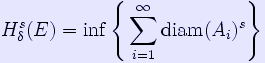
The above example suggests that we can define a set A to have Hausdorff dimension s if its s-dimensional Hausdorff measure is positive and finite; in fact we have to modify this slightly. The Hausdorff dimension of A is the cutoff value s where below s the s-dimensional Hausdorff measure is ∞ and above s it is 0. It is possible for the s dimensional Hausdorff measure of an s dimensional set to be 0 or ∞. For instance R has dimension 1 and its 1-dimensional Hausdorff measure is infinite. To carry this construction of this measure, we use a theory of measure which is appropriate for metric spaces. Define a family of metric outer measures on X using the Method II construction of outer measures due to Munroe and described in the article outer measure. Let C be the class of all subsets of X; for each positive real number s, let ps be the function A → diam(A)s on C. The Hausdorff outer measure of dimension s, denoted Hs, is the outer measure corresponding to the function ps on C. Thus, for any subset E of X where the infimum is taken over sequences {Ai}i which cover E by sets each with diameter ≤ δ. This quantity is non-decreasing as We can succinctly (though not in a very useful way) describe the value Hs(E) as the infimum of all h > 0 such that for all δ > 0, E can be covered by countably many closed sets of diameter ≤ δ; and the sum of the s-th powers of these diameters is less than or equal to h. The function s → Hs(E) is non-increasing. In fact, it turns out that for all values of s, except possibly one Hs(E) is either 0 or ∞. We say E has positive finite Hausdorff dimension if, and only if, there is a real number 0<d< ∞ such that if s < d then Hs(E) = ∞ and if s > d, then Hs(E) = 0. If Hs(E)=0 for all positive s, then E has Hausdorff dimension 0. Finally, if Hs(E)=∞ for all positive s, then E has Hausdorff dimension ∞. In other words,
It is clear from the definition that any metric space has been assigned a dimension in the range [0,∞]. It is also easy to check that Hausdorff dimension is a bi-Lipschitz invariant of metric spaces (see below). Results The Hausdorff outer measure Hs is defined for all subsets of X. However, we can in general assert additivity properties, that is
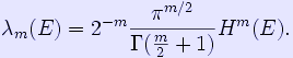
for disjoint A, B, only when A and B satisfy some additional condition, such as both being Borel sets (or more generally, that they are both measurable sets). From the perspective of assigning measure and dimension to sets with unusual metric properties such as fractals, however, this is not a restriction. Theorem. Hs is a metric outer measure. Thus all Borel subsets of X are measurable and Hs is a countably additive measure on the σ-algebra of Borel sets. Clearly, if (X, d) and (Y, e) are isomorphic metric spaces, then the corresponding Hausdorff measure spaces are also isomorphic. It is more useful to note however that Hausdorff measure even behaves well under certain bounded modifications of the underlying metric. Hausdorff measure is a Lipschitz invariant in the following sense: If d and d1 are metrics on X such that for some 0< C < ∞ and all x, y in X, then the corresponding Hausdorff measures Hs, H1s satisfy for any Borel set E. Note that if m is a positive integer, the m dimensional Hausdorff measure of Rn is a rescaling of usual m-dimensional Lebesgue measure λm which is normalized so that the Lebesgue measure of the m-dimensional unit cube [0,1]m is 1. In fact, for any Borel set E, Remark. Some authors adopt a slightly different definition of Hausdorff measure than the one chosen here, the difference being that it is normalized in such a way that Hausdorff m-dimensional measure in the case of Euclidean space coincides exactly with the Lebesgue measure λ. See the Federer reference below for additional material on other fractal measures. Examples * The Euclidean space Rn has Hausdorff dimension n. * The circle S1 has Hausdorff dimension 1. * Countable sets have Hausdorff dimension 0. * Fractals often are spaces whose Hausdorff dimension strictly exceeds the topological dimension. For example, the Cantor set (a zero-dimensional topological space) is a union of two copies of itself, each copy shrunk by a factor 1/3; this fact can be used to prove that its Hausdorff dimension is ln2 / ln3, which is approximately 0.63 (see natural logarithm). The Sierpinski triangle is a union of three copies of itself, each copy shrunk by a factor of 1/2; this yields a Hausdorff dimension of ln3 / ln2, which is approximately 1.58. * Spacefilling curves like the Peano and the Sierpiński curve by definition have Hausdorff dimension 2. * The trajectory of Brownian motion in dimension 2 and above has Hausdorff dimension 2 almost surely. * The Hausdorff dimension of many coastlines have been measured, partly due to an early paper by Benoit Mandelbrot entitled How Long Is the Coast of Britain? Statistical Self-Similarity and Fractional Dimension. The results vary from 1.02 for the coastline of South Africa to 1.25 for the west coast of Great Britain. Hausdorff dimension and topological dimension Let X be an arbitrary separable metric space. There is a notion of topological dimension for X which is defined recursively. It is always an integer (or +∞) and is denoted dimtop(X). Theorem. Suppose X is non-empty. Then Moreover
where Y ranges over metric spaces homeomorphic to X. In other words, X and Y have the same underlying set of points and the metric dY of Y is topologically equivalent to dX. These results were originally established by Edward Szpilrajn (1907-1976). The treatment in Chapter VIII of the Hurewicz and Wallman reference is particularly recommended. Self-similar sets Many sets defined by a self-similarity condition have dimensions which can be determined explicitly. Roughly, a set E is self-similar if it is the fixed point of a set-valued transformation ψ, that is ψ(E) = E, although the exact definition is given below. The following is Theorem 8.3 of the Falconer reference below: Theorem. Suppose
are contractive mappings on Rn with contraction constant rj < 1. Then there is a unique non-empty compact set A such that This follows from Stefan Banach's contractive mapping fixed point theorem applied to the complete metric space of non-empty compact subsets of Rn with the Hausdorff distance. To determine the dimension of the self-similar set A (in certain cases), we need a technical condition called the open set condition on the sequence of contractions ψi which is stated as follows: There is a relatively compact open set V such that
where the sets in union on the left are pairwise disjoint. Theorem. Suppose the open set condition holds and each ψi is a similitude, that is a composition of an isometry and a dilation around some point. Then the unique fixed point of ψ is a set whose Hausdorff dimension is s where s is the unique solution of
Note that the contraction coefficient of a similitude is the magnitude of the dilation. We can use this theorem to compute the Hausdorff dimension of the Sierpinski triangle (or sometimes called Sierpinski gasket). Consider three non-collinear points a1, a2, a3 in the plane R² and let ψi be the dilation of ratio 1/2 around ai. The unique non-empty fixed point of the corresponding mapping ψ is a Sierpinski gasket and the dimension s is the unique solution of Taking natural logarithms of both sides of the above equation, we can solve for s, that is:
The Sierpinski gasket is self-similar. In general a set E which is a fixed point of a mapping is self-similar if and only if the intersections where s is the Hausdorff dimension of E. This is clear in the case of the Sierpinski gasket (the intersections are just points), but is also true more generally: Theorem. Under the same conditions as the previous theorem, the unique fixed point of ψ is self-similar. See also * List of fractals by Hausdorff dimension, some examples of deterministic fractals, random and natural fractals Historical references * A. S. Besicovitch, On Linear Sets of Points of Fractional Dimensions, Mathematische Annalen 101 (1929). * A. S. Besicovitch and H. D. Ursell, Sets of Fractional Dimensions, Journal of the London Mathematical Society, v12 (1937). Several selections from this volume are reprinted in Classics on Fractals,ed. Gerald A. Edgar, Addison-Wesley (1993) ISBN 0-201-58701-7 See chapters 9,10,11. * F. Hausdorff, Dimension und äußeres Maß, Mathematische Annalen 79(1–2) (March 1919) pp. 157–179. References 1. ^ Mandelbrot, Benoît (1982). The Fractal Geometry of Nature, Lecture notes in mathematics 1358. W. H. Freeman. ISBN 0716711869. * M. Maurice Dodson and Simon Kristensen, Hausdorff Dimension and Diophantine Approximation (June 12, 2003). Retrieved from "http://en.wikipedia.org/" |
|
 .
.