Dot product

In mathematics, the dot product or scalar product is an algebraic operation that takes two equal-length sequences of numbers (usually coordinate vectors) and returns a single number obtained by multiplying corresponding entries and then summing those products. The name "dot product" is derived from the centered dot " \( \cdot \) " that is often used to designate this operation; the alternative name "scalar product" emphasizes the scalar (rather than vector) nature of the result.

When two Euclidean vectors are expressed in terms of coordinate vectors on an orthonormal basis, the inner product of the former is equal to the dot product of the latter. For more general vector spaces, while both the inner and the dot product can be defined in different contexts (for instance with complex numbers as scalars) their definitions in these contexts may not coincide.

In three dimensional space, the dot product contrasts with the cross product, which produces a vector as result. The dot product is directly related to the cosine of the angle between two vectors in Euclidean space of any number of dimensions.

Definition

The dot product of two vectors a = [a1, a2, ..., an] and b = [b1, b2, ..., bn] is defined as:

\( \mathbf{a}\cdot \mathbf{b} = \sum_{i=1}^n a_ib_i = a_1b_1 + a_2b_2 + \cdots + a_nb_n \)

where Σ denotes summation notation and n is the dimension of the vector space.

In dimension 2, the dot product of vectors [a,b] and [c,d] is ac + bd. Similarly, in a dimension 3, the dot product of vectors [a,b,c] and [d,e,f] is ad + be + cf. For example, the dot product of two three-dimensional vectors [1, 3, −5] and [4, −2, −1] is

\( [1, 3, -5] \cdot [4, -2, -1] = (1)(4) + (3)(-2) + (-5)(-1) = 4 - 6 + 5 = 3. \)

Given two column vectors, their dot product can also be obtained by multiplying the transpose of one vector with the other vector and extracting the unique coefficient of the resulting 1 × 1 matrix. The operation of extracting the coefficient of such a matrix can be written as taking its determinant or its trace (which is the same thing for 1 × 1 matrices); since in general tr(AB) = tr(BA) whenever AB or equivalently BA is a square matrix, one may write

\( \mathbf{a} \cdot \mathbf{b} = \det( \mathbf{a}^{\mathrm{T}}\mathbf{b} ) = \det( \mathbf{b}^{\mathrm{T}}\mathbf{a} ) = \mathrm{tr} ( \mathbf{a}^{\mathrm{T}}\mathbf{b} ) = \mathrm{tr} ( \mathbf{b}^{\mathrm{T}}\mathbf{a} ) = \mathrm{tr} ( \mathbf{a}\mathbf{b}^{\mathrm{T}} ) = \mathrm{tr} ( \mathbf{b}\mathbf{a}^{\mathrm{T}} ) \)

More generally the coefficient (i,j) of a product of matrices is the dot product of the transpose of row i of the first matrix and column j of the second matrix.

Geometric interpretation

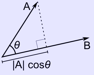
\( \mathbf{A}_B = \left\|\mathbf{A}\right\| \cos\theta \) is the scalar projection of \( \mathbf{A} \) onto \( \mathbf{B}. \)
Since \( \mathbf{A} \cdot \mathbf{B} = \left\|\mathbf{A}\right\| \left\|\mathbf{B}\right\| \cos\theta, then \mathbf{A}_B = \frac{\mathbf{A} \cdot \mathbf{B}}{\left\|\mathbf{B}\right\|}. \)

In Euclidean geometry, the dot product of vectors expressed in an orthonormal basis is related to their length and angle. For such a vector \( \mathbf{a} \), the dot product \( \mathbf{a}\cdot\mathbf{a} \) is the square of the length (magnitude) of \( \mathbf{a} \) , denoted by \( \left\|\mathbf{a}\right\| \):

\( {\mathbf{a} \cdot \mathbf{a}}=\left\|\mathbf{a}\right\|^2 \)

If \mathbf{b} is another such vector, and \theta is the angle between them:

\( \mathbf{a} \cdot \mathbf{b}=\left\|\mathbf{a}\right\| \, \left\|\mathbf{b}\right\| \cos \theta \, \)

This formula can be rearranged to determine the size of the angle between two nonzero vectors:

\( \theta=\arccos \left( \frac {\bold{a}\cdot\bold{b}} {\left\|\bold{a}\right\|\left\|\bold{b}\right\|}\right). \)

The Cauchy–Schwarz inequality guarantees that the argument of \( \arccos \) is valid.

One can also first convert the vectors to unit vectors by dividing by their magnitude:

\( \boldsymbol{\hat{a}} = \frac{\bold{a}}{\left\|\bold{a}\right\|} \)

then the angle \theta is given by

\( \theta = \arccos ( \boldsymbol{\hat a}\cdot\boldsymbol{\hat b}). \)

The terminal points of both unit vectors lie on the unit circle. The unit circle is where the trigonometric values for the six trig functions are found. After substitution, the first vector component is cosine and the second vector component is sine, i.e. \( (\cos x, \sin x) \) for some angle x. The dot product of the two unit vectors then takes (\cos x, \sin x) and (\cos y, \sin y) \) for angles x and y and returns \( \cos x \, \cos y + \sin x \, \sin y = \cos(x - y) \) where \( x - y = \theta. \)

As the cosine of 90° is zero, the dot product of two orthogonal vectors is always zero. Moreover, two vectors can be considered orthogonal if and only if their dot product is zero, and they have non-null length. This property provides a simple method to test the condition of orthogonality.

Sometimes these properties are also used for "defining" the dot product, especially in 2 and 3 dimensions; this definition is equivalent to the above one. For higher dimensions the formula can be used to define the concept of angle.

The geometric properties rely on the basis being orthonormal, i.e. composed of pairwise perpendicular vectors with unit length.
Scalar projection

If both \( \mathbf{a} \) and \( \mathbf{b} \) have length one (i.e., they are unit vectors), their dot product simply gives the cosine of the angle between them.

If only \( \mathbf{b} \) is a unit vector, then the dot product \( \mathbf{a}\cdot\mathbf{b} \) gives \( \left\|\mathbf{a}\right\|\cos\theta \) , i.e., the magnitude of the projection of \( \mathbf{a} \) in the direction of \( \mathbf{b} \) , with a minus sign if the direction is opposite. This is called the scalar projection of \( \mathbf{a} \) onto \( \mathbf{b} \) , or scalar component of \( \mathbf{a} \) in the direction of \( \mathbf{b} \) (see figure). This property of the dot product has several useful applications (for instance, see next section).

If neither \( \mathbf{a} nor \( \mathbf{b} is a unit vector, then the magnitude of the projection of \mathbf{a} in the direction of \( \mathbf{b} is \( \mathbf{a}\cdot\frac{\mathbf{b}}{\left\|\mathbf{b}\right\|} \) , as the unit vector in the direction of \( \mathbf{b} is \frac{\mathbf{b}}{\left\|\mathbf{b}\right\|}. \)

Rotation

When an orthonormal basis that the vector \mathbf{a} is represented in terms of is rotated, \mathbf{a}'s matrix in the new basis is obtained through multiplying \mathbf{a} by a rotation matrix \mathbf{R}. This matrix multiplication is just a compact representation of a sequence of dot products.

For instance, let

\( \mathbf{B}_1 = \{\mathbf{x}, \mathbf{y}, \mathbf{z}\} and \mathbf{B}_2 = \{\mathbf{u}, \mathbf{v}, \mathbf{w}\} \) be two different orthonormal bases of the same space \( \mathbb{R}^3, with \mathbf{B}_2 \) obtained by just rotating \( \mathbf{B}_1, \)
\( \mathbf{a}_1 = (a_x, a_y, a_z) \) represent vector \mathbf{a} in terms of \mathbf{B}_1,
\( \mathbf{a}_2 = (a_u, a_v, a_w) \) represent the same vector in terms of the rotated basis \( \mathbf{B}_2, \)
\( \mathbf{u}_1, \mathbf{v}_1, \mathbf{w}_1, \) be the rotated basis vectors \( \mathbf{u}, \mathbf{v}, \mathbf{w} represented in terms of \mathbf{B}_1. \)

Then the rotation from \( \mathbf{B}_1 to \mathbf{B}_2 \) is performed as follows:

\( \bold a_2 = \bold{Ra}_1 = \begin{bmatrix} u_x & u_y & u_z \\ v_x & v_y & v_z \\ w_x & w_y & w_z \end{bmatrix} \begin{bmatrix} a_x \\ a_y \\ a_z \end{bmatrix} = \begin{bmatrix} \bold u_1\cdot\bold a_1 \\ \bold v_1\cdot\bold a_1 \\ \bold w_1\cdot\bold a_1 \end{bmatrix} = \begin{bmatrix} a_u \\ a_v \\ a_w \end{bmatrix} . \)

Notice that the rotation matrix \( \mathbf{R} \) is assembled by using the rotated basis vectors \( \mathbf{u}_1, \mathbf{v}_1, \mathbf{w}_1 \) as its rows, and these vectors are unit vectors. By definition, \( \mathbf{Ra}_1 \) consists of a sequence of dot products between each of the three rows of \( \mathbf{R} \) and vector \( \mathbf{a}_1 \) . Each of these dot products determines a scalar component of \( \mathbf{a} \) in the direction of a rotated basis vector (see previous section).

If \( \mathbf{a}_1 is a row vector, rather than a column vector, then \( \mathbf{R} \) must contain the rotated basis vectors in its columns, and must post-multiply \( \mathbf{a}_1 \) :

\( \bold a_2 = \bold a_1 \bold R = \begin{bmatrix} a_x & a_y & a_z \end{bmatrix} \begin{bmatrix} u_x & v_x & w_x \\ u_y & v_y & w_y \\ u_z & v_z & w_z \end{bmatrix} = \begin{bmatrix} \bold u_1\cdot\bold a_1 & \bold v_1\cdot\bold a_1 & \bold w_1\cdot\bold a_1 \end{bmatrix} = \begin{bmatrix} a_u & a_v & a_w \end{bmatrix} . \)

Physics

In physics, vector magnitude is a scalar in the physical sense, i.e. a physical quantity independent of the coordinate system, expressed as the product of a numerical value and a physical unit, not just a number. The dot product is also a scalar in this sense, given by the formula, independent of the coordinate system. Example:

Mechanical work is the dot product of force and displacement vectors.
Magnetic flux is the dot product of the magnetic field and the area vectors.

Properties

The following properties hold if a, b, and c are real vectors and r is a scalar.

The dot product is commutative:

\( \mathbf{a} \cdot \mathbf{b} = \mathbf{b} \cdot \mathbf{a}. \)

The dot product is distributive over vector addition:

\( \mathbf{a} \cdot (\mathbf{b} + \mathbf{c}) = \mathbf{a} \cdot \mathbf{b} + \mathbf{a} \cdot \mathbf{c}. \)

The dot product is bilinear:

\( \mathbf{a} \cdot (r\mathbf{b} + \mathbf{c}) = r(\mathbf{a} \cdot \mathbf{b}) +(\mathbf{a} \cdot \mathbf{c}). \)

When multiplied by a scalar value, dot product satisfies:

\( (c_1\mathbf{a}) \cdot (c_2\mathbf{b}) = (c_1c_2) (\mathbf{a} \cdot \mathbf{b}) \)

(these last two properties follow from the first two).

Two non-zero vectors a and b are orthogonal if and only if a • b = 0.

Unlike multiplication of ordinary numbers, where if ab = ac, then b always equals c unless a is zero, the dot product does not obey the cancellation law:

If a • b = a • c and a ≠ 0, then we can write: a • (b − c) = 0 by the distributive law; the result above says this just means that a is perpendicular to (b − c), which still allows (b − c) ≠ 0, and therefore b ≠ c.

Provided that the basis is orthonormal, the dot product is invariant under isometric changes of the basis: rotations, reflections, and combinations, keeping the origin fixed. The above mentioned geometric interpretation relies on this property. In other words, for an orthonormal space with any number of dimensions, the dot product is invariant under a coordinate transformation based on an orthogonal matrix. This corresponds to the following two conditions:

The new basis is again orthonormal (i.e., it is orthonormal expressed in the old one).
The new base vectors have the same length as the old ones (i.e., unit length in terms of the old basis).

If a and b are functions, then the derivative of a • b is a' • b + a • b'
Triple product expansion
Main article: Triple product

This is a very useful identity (also known as Lagrange's formula) involving the dot- and cross-products. It is written as

\( \mathbf{a} \times (\mathbf{b} \times \mathbf{c}) = \mathbf{b}(\mathbf{a}\cdot\mathbf{c}) - \mathbf{c}(\mathbf{a}\cdot\mathbf{b}) \)

which is easier to remember as "BAC minus CAB", keeping in mind which vectors are dotted together. This formula is commonly used to simplify vector calculations in physics.
Proof of the geometric interpretation

Consider the element of Rn

\( \mathbf{v} = v_1 \mathbf{\hat{e}}_1 + v_2 \mathbf{\hat{e}}_2 + ... + v_n \mathbf{\hat{e}}_n. \, \)

Repeated application of the Pythagorean theorem yields for its length |v|

\( |\mathbf{v}|^2 = v_1^2 + v_2^2 + ... + v_n^2. \, \)

But this is the same as

\( \mathbf{v} \cdot \mathbf{v} = v_1^2 + v_2^2 + ... + v_n^2, \, \)

so we conclude that taking the dot product of a vector v with itself yields the squared length of the vector.

Lemma 1
\( \mathbf{v} \cdot \mathbf{v} = |\mathbf{v}|^2. \, \)

Now consider two vectors a and b extending from the origin, separated by an angle θ. A third vector c may be defined as

\( \mathbf{c} \ \stackrel{\mathrm{def}}{=}\ \mathbf{a} - \mathbf{b}. \, \)

creating a triangle with sides a, b, and c. According to the law of cosines, we have

\( |\mathbf{c}|^2 = |\mathbf{a}|^2 + |\mathbf{b}|^2 - 2 |\mathbf{a}||\mathbf{b}| \cos \theta. \, \)

Substituting dot products for the squared lengths according to Lemma 1, we get

\( \mathbf{c} \cdot \mathbf{c} = \mathbf{a} \cdot \mathbf{a} + \mathbf{b} \cdot \mathbf{b} - 2 |\mathbf{a}||\mathbf{b}| \cos\theta. \, \) (1)

But as c ≡ a − b, we also have

\( \mathbf{c} \cdot \mathbf{c} = (\mathbf{a} - \mathbf{b}) \cdot (\mathbf{a} - \mathbf{b}) \,, \)

which, according to the distributive law, expands to

\mathbf{c} \cdot \mathbf{c} = \mathbf{a} \cdot \mathbf{a} + \mathbf{b} \cdot \mathbf{b} -2(\mathbf{a} \cdot \mathbf{b}). \, \) (2)

Merging the two c • c equations, (1) and (2), we obtain

\( \mathbf{a} \cdot \mathbf{a} + \mathbf{b} \cdot \mathbf{b} -2(\mathbf{a} \cdot \mathbf{b}) = \mathbf{a} \cdot \mathbf{a} + \mathbf{b} \cdot \mathbf{b} - 2 |\mathbf{a}||\mathbf{b}| \cos\theta. \, \)

Subtracting a • a + b • b from both sides and dividing by −2 leaves

\( \mathbf{a} \cdot \mathbf{b} = |\mathbf{a}||\mathbf{b}| \cos\theta. \, \)

Q.E.D.
Generalization
Real vector spaces

The inner product generalizes the dot product to abstract vector spaces over the real numbers and is usually denoted by \langle\mathbf{a}\, , \mathbf{b}\rangle. More precisely, if V is a vector space over \mathbb{R}, the inner product is a function V\times V \rightarrow \mathbb{R}. Owing to the geometric interpretation of the dot product, the norm ||a|| of a vector a in such an inner product space is defined as

\( \|\mathbf{a}\| = \sqrt{\langle\mathbf{a}\, , \mathbf{a}\rangle} \)

such that it generalizes length, and the angle θ between two vectors a and b by

\( \cos{\theta} = \frac{\langle\mathbf{a}\, , \mathbf{b}\rangle}{\|\mathbf{a}\| \, \|\mathbf{b}\|}. \)

In particular, two vectors are considered orthogonal if their inner product is zero

\( \langle\mathbf{a}\, , \mathbf{b}\rangle = 0. \)

Complex vectors

For vectors with complex entries, using the given definition of the dot product would lead to quite different geometric properties. For instance the dot product of a vector with itself can be an arbitrary complex number, and can be zero without the vector being the zero vector; this in turn would have severe consequences for notions like length and angle. Many geometric properties can be salvaged, at the cost of giving up the symmetric and bilinear properties of the scalar product, by alternatively defining

\( \mathbf{a}\cdot \mathbf{b} = \sum{a_i \overline{b_i}} \)

where bi is the complex conjugate of bi. Then the scalar product of any vector with itself is a non-negative real number, and it is nonzero except for the zero vector. However this scalar product is not linear in b (but rather conjugate linear), and the scalar product is not symmetric either, since

\( \mathbf{a} \cdot \mathbf{b} = \overline{\mathbf{b} \cdot \mathbf{a}}. \)

The angle between two complex vectors is then given by

\( \cos\theta = \frac{\operatorname{Re}(\mathbf{a}\cdot\mathbf{b})}{\|\mathbf{a}\|\,\|\mathbf{b}\|}. \)

This type of scalar product is nevertheless quite useful, and leads to the notions of Hermitian form and of general inner product spaces.

The Frobenius inner product generalizes the dot product to matrices. It is defined as the sum of the products of the corresponding components of two matrices having the same size.
Generalization to tensors

The dot product between a tensor of order n and a tensor of order m is a tensor of order n+m-2. The dot product is calculated by multiplying and summing across a single index in both tensors. If \mathbf{A} and \( \mathbf{B} are two tensors with element representation \( A_{ij\dots}^{k\ell\dots} and B_{mn\dots}^{p{\dots}i} the elements of the dot product \( \mathbf{A} \cdot \mathbf{B} are given by

\( A_{ij\dots}^{k\ell\dots}\cdot B_{mn\dots}^{p{\dots}i} = \sum_{i=1}^n A_{ij\dots}^{k\ell\dots}B_{mn\dots}^{p{\dots}i}. \)

This definition naturally reduces to the standard vector dot product when applied to vectors, and matrix multiplication when applied to matrices .

Occasionally, a double dot product is used to represent multiplying and summing across two indices. The double dot product between two 2nd order tensors is a scalar quantity.