Mandeltbrot Set Computer drawings Algorithms : * Escape time algorithm o boolean version ( draws M-set and its exterior using 2 colours ) = Mandelbrot algorithm o discrete (integer) version = level set method ( LSM/M ); draws Mandelbrot set and colour bands in its exterior o continuous version o level curves version = draws lemniscates of Mandelbrot set = boundaries of Level Sets[12] o decomposition of exterior of Mandelbrot set * complex potential o Hubbard-Douady (real) potential of Mandelbrot set (CPM/M) - radial part of complex potential o external angle of Mandelbrot set - angular part of complex potential o abstract M-set * Distance estimation method for Mandelbrot set o exterior distance estimation= Milnor algorithm (DEM/M) o interior distance estimation * algorithm used to explore interior of Mandelbrot set o period of hyperbolic components o multiplier of periodic orbit ( internal rays(angle) and intenal radius ) o bof61 and bof60 Every algorithm can be implemented in sequential or parallel version. Mirror symmetry can be used to speed-up calculations. Escape time algorithm The simplest algorithm for generating a representation of the Mandelbrot set is known as the "escape time" algorithm. A repeating calculation is performed for each x, y point in the plot area and based on the behaviour of that calculation, a colour is chosen for that pixel. The x and y location of each point are used as starting values in a repeating, or iterating calculation (described in detail below). The result of each iteration is used as the starting values for the next. The values are checked during each iteration to see if they have reached a critical 'escape' condition. If that condition is reached, the calculation is stopped, the pixel is drawn, and the next x, y point is examined. For some starting values, escape occurs quickly, after only a small number of iterations. For other starting values, it may take hundreds or thousands of iterations to escape. For values within the Mandelbrot set, escape will never occur. The programmer or user must choose how much iteration, or 'depth,' they wish to examine. The higher the maximum number of iterations, the more detail and subtlety emerge in the final image, but the longer time it will take to calculate the picture. The colour of each point represents how quickly the values reached the escape point. Often black is used to show values that fail to escape before the iteration limit, and gradually brighter colours are used for points that escape. This gives a visual representation of how many cycles were required before reaching the escape condition. For programmers The definition of the Mandelbrot set, together with its basic properties, suggests a simple algorithm for drawing a picture of the Mandelbrot set. The region of the complex plane we are considering is subdivided into a certain number of pixels. To colour any such pixel, let c\, be the midpoint of that pixel. We now iterate the critical value c\, under P_c\,, checking at each step whether the orbit point has modulus larger than 2. If this is the case, we know that the midpoint does not belong to the Mandelbrot set, and we colour our pixel. (Either we colour it white to get the simple mathematical image or colour it according to the number of iterations used to get the well-known colourful images). Otherwise, we keep iterating for a certain (large, but fixed) number of steps, after which we decide that our parameter is "probably" in the Mandelbrot set, or at least very close to it, and colour the pixel black. In pseudocode, this algorithm would look as follows.
For each pixel on the screen do:
{
  x = x0 = x co-ordinate of pixel
  y = y0 = y co-ordinate of pixel

  iteration = 0
  max_iteration = 1000

  while ( x*x + y*y <= (2*2)  AND  iteration < max_iteration )
  {

    xtemp = x*x - y*y + x0
    y = 2*x*y + y0

    x = xtemp

    iteration = iteration + 1
  }

  if ( iteration == max_iteration )
  then
    colour = black
  else
    colour = iteration

  plot(x0,y0,colour)
where, relating the pseudocode to c\, , z\, and P_c\,: * z = x + iy * z2 = x2 + i2xy − y2 * c = x0 + iy0 and so, as can be seen in the pseudocode in the computation of x and y: * x = Re(z2 + c) = x2 − y2 + x0 and y = Im(z2 + c) = 2xy + y0 To get colourful images of the set, the assignment of a colour to each value of the number of executed iterations can be made using one of a variety of functions (linear, exponential, etc). One practical way to do it, without slowing down the calculations, is to use the number of executed iterations as an entry to a look-up colour palette table initialized at startup. If the colour table has, for instance, 500 entries, then you can use n mod 500, where n is the number of iterations, to select the colour to use. You can initialize the colour palette matrix in various different ways, depending on what special feature of the escape behavior you want to emphasize graphically. Continuous (smooth) coloring The Escape Time Algorithm is popular for its simplicity. However, it creates bands of color, which can detract from an image's value. This can be fixed using the Normalized Iteration Count Algorithm[13], which provides a smooth transition of colors between iterations. The equation is where n is the number of iterations for z, B is the bailout radius (it is normally 2 for a Mandelbrot set, but it can be changed), and P is the power for which z is raised to in the Mandelbrot set equation (zn+1=znP+c, P is generally 2). Another equation for this is
Note that this new equation is simpler than the first, but it only works for Mandelbrot set's with a bailout radius of 2 and a power of 2.
This image was rendered with the Escape Time Algorithm. Notice the very obvious "bands" of color.
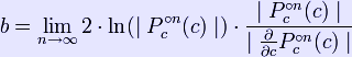
This image was rendered with the Normalized Iteration Count Algorithm. Notice the bands of color have been replaced by a smooth gradient. While this algorithm is relatively simple to implement (using either equation), there are a few things that need to be taken into consideration. First, the two equations return a continuous stream of numbers. However, it is up to you to decide on how the return values will be converted into a color. Some type of method for casting these numbers onto a gradient should be developed. Second, it is recommended that a few extra iterations are done so that z can grow. If you stop iterating as soon as z escapes, there is the possibility that the smoothing algorithm will not work. Distance estimates One can compute distance from point c ( in exterior or interior ) to nearest point on the boundary of Mandelbrot set. Exterior distance estimation The proof of the connectedness of the Mandelbrot set in fact gives a formula for the uniformizing map of the complement of M (and the derivative of this map). By the Koebe 1/4-theorem, one can then estimate the distance between the mid-point of our pixel and the Mandelbrot set up to a factor of 4. In other words, provided that the maximal number of iterations is sufficiently high, one obtains a picture of the Mandelbrot set with the following properties: 1. Every pixel which contains a point of the Mandelbrot set is coloured black. 2. Every pixel which is colored black is close to the Mandelbrot set. he distance estimate of a pixel c (a complex number) from the Mandelbrot set is given by
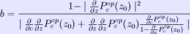
where * * * From a mathematician's point of view, this formula only works in limit where n goes to infinity, but very reasonable estimates can be found with just a few additional iterations after the main loop exits. Once b is found, by the Koebe 1/4-theorem, we know there's no point of the Mandelbrot set with distance from c smaller than b/4. Interior distance estimation It is also possible to estimate the distance of a limitly periodic (i.e., inner) point to the boundary of the Mandelbrot set. The estimate is given by where * p is the period, * c is the point to be estimated, * Pc(z) is the complex quadratic polynomial Pc(z) = z2 + c * * z0 is any of the p points that make the attractor of the iterations of * Given p and z0, * * \ Analogous to the exterior case, once b is found, we know that all points within the distance of b/4 from c are inside the Mandelbrot set. There are two practical problems with the interior distance estimate: first, we need to find z0 precisely, and second, we need to find p precisely. The problem with z0 is that the convergence to z0 by iterating Pc(z) requires, theoretically, an infinite number of operations. The problem with period is that, sometimes, due to rounding errors, a period is falsely identified to be an integer multiple of the real period (e.g., a period of 86 is detected, while the real period is only 43=86/2). In such case, the distance is overestimated, i.e., the reported radius could contain points outside the Mandelbrot set. Optimizations One way to improve calculations is to find out beforehand whether the given point lies within the cardioid or in the period-2 bulb. To prevent having to do huge numbers of iterations for other points in the set, one can do "periodicity checking"—which means check if a point reached in iterating a pixel has been reached before. If so, the pixel cannot diverge, and must be in the set. This is most relevant for fixed-point calculations, where there is a relatively high chance of such periodicity—a full floating-point (or higher-accuracy) implementation would rarely go into such a period. Periodicity checking is, of course, a trade-off: The need to remember points costs memory and data management instructions, whereas it saves computational instructions Retrieved from "http://en.wikipedia.org/" |
|


 .
.